Python: Co-variance and Correlation

In this lesson, I will using data from a CSV file. You can download the file here: heightWeight

If you do not know how to import CSV files into Python, check out my lesson on it first: Python: Working with CSV Files

The Data

The data set includes 20 heights (inches) and weights(pounds). Given what you already know, you could tell me the average height and average weight. You could tell me medians, variances and standard deviations.

correl

But all of those measurements are only concerned with a single variable. What if I want to see how height interacts with weight? Does weight increase as height increases?

**Note while there are plenty of fat short people and overly skinny tall people, when you look at the population at large, taller people will tend to weigh more than shorter people. This generalization of information is very common as it gives you a big picture view and is not easily skewed by outliers.

Populate Python with Data

The first thing we are going to focus on is co-variance. Let’s start by getting our data in Python.

correl1.jpg

Now there is a small problem. Our lists are filled with strings, not numbers. We can’t do calculations on strings.

We can fix this by populating converting the values using int(). Below I created 2 new lists (height and weight), created a for loop counting up to number of values in our lists : range(len(hgt)). Then I filled the new lists using lst.append(int(value))

correl2.jpg

**Now I know I could have resolved this in fewer steps, but this is a tutorial, so I want to provide more of a walk through.

Co-variance

Co-variance tells us how much two variables disperse from the mean together. There are multiple ways to find co-variance, but for me, using a dot product approach has always been the simplest.

For those unfamiliar with dot product. Imagine I had 2 lists (a,b) with 4 elements each. The dot product with calculated as so: a[0]*b[0]+a[1]*b[1]+a[2]*b[2]+a[3]*b[3]

Here is how it works:

If I take the individual variance of height[0] and weight[0] and they are both positive or negative – the product will be positive. – both variables are moving in the same direction

One positive and one negative will be negative. The variables are moving in different directions

One you add them all up, a positive number will mean that overall, you variables seem to have a positive co-variance (if a goes up, b goes up – if a goes down, b goes down)

If the final result is negative, you have negative co-variance (if a goes up, b goes down – if a goes down, b goes up)

If your final answer is 0 – your variables have no measurable interaction

Okay, let’s program this thing

** we will be using numpy’s mean() – mean and dot() – dot product methods and corrcoef() – correlation coefficient

First we need to find the individual variances from mean for each list

I create a function called ind_var that uses a list comprehension to subtract the mean from each element in the list.

correl3.jpg

Now, let’s change out the print statement for a return, because we are going to be using this function inside another function.

correl4.jpg

Co-variance function

Now let’s build the co-variance function. Here we are taking the dot product of the variances of each element of height and weight. We then divide the result by the N-1 (the number of elements – 1 : the minus 1 is due to the fact we are dealing with sample data not population)

correl6

So what were are doing:

  • Take the first height (68 inches) and subtract the mean (66.8) from it (1.2)
  • Take the first weight (165 lbs) and subtract the mean(165.8)  from it (-0.8)
  • We then multiply these values together (-0.96)
  • We repeat this for each element
  • Add the elements up.
  • Divide by 19 (20-1)
  • 144.75789 is our answer

Our result is 144.75789  – a positive co-variance. So when height goes up – weight goes up, when height goes down – weight goes down.

But what does 144 mean? Not much unfortunately. The co-variance doesn’t relate any information as to what units we are working with. 144 miles is a long way, 144 cm not so much.

Correlation

So we have another measurement known as correlation. A very basic correlation equation divides out the standard deviation of both height and weight. The result of a correlation is between 1 and -1. With -1 being perfect anti-correlation and 1 being perfect correlation. 0 mean no correlation exists.

With my equation get 1.028  – more than one. This equation is simplistic and prone to some error.

correl7.jpg

numpy’s corrcoef() is more accurate. It shows us a correlation matrix. Ignore the 1’s – they are part of what is known as the identity. Instead look at the other numbers = 0.97739.  That is about as close to one as you will ever get in reality. So even if my equation is off, it isn’t too far off.

correl9

Now just to humor me. Create another list to play with.

correl10

Let’s run this against height in my correlation function

correl11.jpg

Run these value through the more accurate corrcoef() . This will show my formula is still a bit off, but for the most part, it is not all that bad.

correl8


If you enjoyed this lesson, click LIKE below, or even better, leave me a COMMENT. 

Follow this link for more Python content: Python


Python: Central Limit Theorem

The Central Limit Theorem is one of core principles of probability and statistics. So much so, that a good portion of inferential statistical testing is built around it. What the Central Limit Theorem states is that, given a data set – let’s say of 100 elements (See below) if I were to take a random sampling of 10 data points from this sample and take the average (arithmetic mean) of this sample and plot the result on a histogram, given enough samples my histogram would approach what is known as a normal bell curve.

In plain English

  • Take a random sample from your data
  • Take the average of your sample
  • Plot your sample on a histogram
  • Repeat 1000 times
  • You will have what looks like a normal distribution bell curve when you are done.

hist4

For those who don’t know what a normal distribution bell  curve looks like, here is an example. I created it using numpy’s normal method

hist5.jpg

If you don’t believe me, or want to see a more graphical demonstration – here is a link to a simulation that helps a lot of people to grasp this concept: link

Okay, I have bell curve, who cares?

The normal distribution of (Gaussian Distribution – named after the mathematician Carl Gauss) is an amazing statistical tool. This is the powerhouse behind inferential statistics.

The Central Limit Theorem tells me (under certain circumstances), no matter what my population distribution looks like, if I take enough means of sample sets, my sample distribution will approach a normal bell curve.

Once I have a normal bell curve, I now know something very powerful.

Known as the 68,95,99 rule, I know that 68% of my sample is going to be within one standard deviation of the mean. 95% will be within 2 standard deviations and 99.7% within 3.

hist.jpg

So let’s apply this to something tangible. Let’s say I took random sampling of heights for adult men in the United States. I may get something like this (warning, this data is completely made up – do not even cite this graph as anything but bad art work)

hist6.jpg

But reading this graph, I can see that 68% of men are between 65 and 70 inches tall. While less than 0.15% of men are shorter than 55 inches or taller than 80 inches.

Now, there are plenty of resources online if you want to dig deeper into the math. However, if you just want to take my word for it and move forward, this is what you need to take away from this lesson:

p value

As we move into statistical testing like Linear Regression, you will see that we are focus on a p value. And generally, we want to keep that p value under 0.5. The purple box below shows a p value of 0.5 – with 0.25 on either side of the curve. A finding with a p value that low basically states that there is only a 0.5% chance that the results of whatever test you are running are a result of random chance. In other words, your results are 99% repeatable and your test demonstrates statistical significance.

hist7.jpg

Python: Arithmetic, Relational Operators, and Variables

Arithmetic Operators

Python Arithmetic Operators are pretty standard.

Arithmetic Operators

  • + : Addition
  • – : Subtraction
  • * : Multiplication
  • / : Division
  • //: Integer Division (Return divisor: 5/2 = 2)
  • % : Modulus (returns the remainder of a division problem: 5%2=1)
  • ** : Exponent (4**2 = 16)

Screenshot 2022-07-05 124159

Try your code in our online Python console: 

Relational Operators

Relational operators compare values and return a Boolean result (Boolean means 2 states, in this case True or False). Note when using relational operators, == is equal to. A single = is used to set a variable value, not to compare two values

> Greater than

< Less Than 

== Equal to

!= not equal

>= or <= greater than or equal, less than or equal

Screenshot 2022-07-05 122503

Try your code in our online Python console: 

Variables

Variables are a way of holding values in a program. You take a unique character string and you can assign values to it, and use the string throughout your program. Variables in Python are pretty straight forward. Unlike other programming languages, you do not need to define the variables first. Python dynamically assigns the data type.

Three main rules:

  • Variables must start with a letter or _
  • Variables are case sensitive
  • Avoid using command keywords (print, def, for)

pythonFundamentals3

notice lowercase ‘a‘ returns an error

Remember, Jupyter notebooks only return the last command. If you want both variables, use the print command

Screenshot 2022-07-03 210654

You can perform arithmetic functions on variables

Screenshot 2022-07-03 211010

And of course, variables can hold strings as well

Screenshot 2022-07-05 122935

Try your code in our online Python console: 

Last Lesson: Install Python and Hello World

Next Lesson: Print Variables and User Input

Back to Python Course: Course

Python: Fun with Central Tendency

Now numpy provides easy functions for finding central tendency – you can find them in my Numpy Part II lesson: Python: Numpy Part II.

But we have learned enough about Python so far, that maybe it would be more fun to build our own functions. In this lesson we are going to build our own statistics library with mean, median, mode, and quantile

Our Data

pythonCent

Mean

pythonCent1.jpg

or even easier:

pythonCent3

Median

Remember with median – if your data contains an odd number of elements (n%2==1), you just take the middle value. However, if your data contains and even number of elements (n%2==0) then you add the two middle numbers and divide by 2.

We handle that through the use of an if statement in our function.

pythonCent2

Mode

For mode, we want to find the most common element in the list. For this task, I will import Counter from collections.

d.most_common() returns each unique element and the number of times it appears

d.most_common(1) returns the

pythonCent4.jpg

or in function form:

pythonCent5.jpg

In my numpy part II lesson I use a more elegant solution, but I want you to see that there is always more than one way to do something in Python.

Quantile

Quantiles are cut points in set of data. They can represent the bottom ten percent of the data or the top 75% or any % from 0 to 100.

In my solution, I am adding a slicing argument to the sorted() function. Below shows all elements up to (but not including) index 4

pythonCent6

quantile function:

pythonCent7


If you enjoyed this lesson, click LIKE below, or even better, leave me a COMMENT. 

Follow this link for more Python content: Python

Python: Pandas, Working with DataFrames

Sure DataFrames look nice, but how can I work with them?

Let’s cover some basic tasks in pandas to get you started.

Let’s start by building a DataFrame

pyDF1

I don’t like where they placed Age on my dataframe. I want to move it.

To do so, we are going to cover a couple of new terms: axis, drop() and insert()

Axis

Using numpy and pandas, you will come across many functions that require you to enter an axis as a parameter. Axis 0 is your rows while Axis 1 is your columns. This is due to the way matrices are named with a 3×2 matrix having 3 rows and 2 columns and a 2×3 having 2 rows and 3 columns

pyDF2

drop()

To move the age column, I am first going to create a copy of my dataframe minus the age column. To do this, I am going to use the drop() function. The drop() function accepts two arguments drop(name, axis). In our case name = ‘Age’ and axis = 1 since we are referring to a column.

pyDF3

insert()

Now we want to insert the age column. The syntax for the insert() function is insert(insert point, name, data)

pyDF4

add a new column

Adding a new column is straight forward. Just DataFrame[new column name] = value.

Below I created at new column called ‘Age When Start’ that shows the age of employees when they started. I derived this value by subtracting Years Service column from Age column.

pyDF5.jpg

boolean column

You can create a boolean column using a boolean operator.

pyDF6

sort()

You can sort a dataframe by any column using sort_values()

pyDF7.jpg

Sort is set to ascending by default. To reverse it, set ascending = False

** remember in Python, True and False need to start with a capital letter.

pyDF8.jpg

slicing

by rows

slicing by rows is just like with a list

pyDF9

by columns

slicing by columns is a bit more complex. To slice by column name you have to use the dataframe.ix command.

pyDF10


If you enjoyed this lesson, click LIKE below, or even better, leave me a COMMENT. 

Last Lesson: Pandas DataFrames

Next Lesson: Pandas: Rename a Column

Return to: Python for Data Science Course

Follow this link for more Python content: Python


Python: Numpy Part II

Beyond numpy’s usefulness in creating arrays and matrices, numpy also provides a great suite of math functions that – for anyone with any programming background – are fairly intuitive.

Here are some examples:

np.pi returns pi and np.sqrt() takes the square root of whatever value you feed it.

pyNp2.jpg

Trig Functions

numpy handles most common trigonometry functions.

pyNp2_1

Stats

Numpy handles many statistics functions.

Below we have mean and median. Unfortunately, just like in R, there is no mode command, but we can fake it using Set.

pyNp2_2

using set to fake mode

pyNp2_4

Numpy can also be used to find range, variance, and standard deviation.

pyNp2_5

Rounding

Numpy has rounding features for dealing with decimals. It also has floor() and ceil() functions that bring the number down to the “floor” or up to the “ceiling”

pyNp2_6

Use in creating graphs

use np.sin()

pyNp2_7.jpg

use np.log()

pyNp2_8

you can even put the two together

pyNp2_9

linspace()

My final one today is a function called linspace(). It lets you create a start and finish point, and how many elements you want. It then will create a even list of number between start and finish.

linspace(start,finish, num=numbers you want)

pyNp2_10


If you enjoyed this lesson, click LIKE below, or even better, leave me a COMMENT. 

Last Lesson: Numpy

Next Lesson: Pandas (Series)

Return to: Python for Data Science Course

Follow this link for more Python content: Python


Python: Create, Import, and Use a Module

Today we are going to cover what I consider a flaw in the iPython Notebook environment. Code you write cannot be imported into another program like you can using just a standard Python compiler. At least it cannot under its native .ipynb format.

For this example, we are going to use the Spyder IDE that comes with Anaconda. You can use any IDE you want, in all honesty, you can use a simple notepad editor to do this if you don’t have Spyder installed.


Create a Module

I am going to create a little module called math_bl.py. This module contains 3 simple functions: sqr2, sub2, and add2


In my instance, my iPython notebooks are stored under my user directory. If you are not sure where you notebooks are, you can use the pwd command (print working directory). This will tell you where to save your math_bl.py file to.

pyModu3.jpg

** note the double \\ are due to a formatting function in Python. \ is a break command that can be used for many purposes. Example \t means to insert a tab.

pyModu4.jpg

So effectively you have to use \\ if you want a \ in Python, making my working directory C:\Users\Benjamin  

Import the Module

Now if I open up a new notebook and try using the functions I have just created, I will error out.

So, what I need to do is import add2, then I can start calling on the functions I created in add2


If you enjoyed this lesson, click LIKE below, or even better, leave me a COMMENT. 

Next Lesson: 

Return to: Python for Data Science Course

Follow this link for more Python content: Python

Python: Error handling

No matter how well crafted your code, you will inevitably come across an error every once in a while. Unfortunately, Python’s default setting when catching an error is to crash the program.

In the example below, I accidentally asked for a letter, when the code int(input()) is looking for an integer.

So when I enter a string, I get an error

Try your code in our online Python console:  

Try

Using Try, we can handle such mishaps in a more elegant fashion

The syntax is a follows:

try:
        Your Code
except: 
         What to do if your code errors out
else:
         What to do if your code is successful

And as you can see from above, it doesn’t just protect against code errors, but it protects against user errors as well.

Using a while loop, we can give the user another chance if they don’t enter a number the first time.

Code explanation

  • while True:  – starts an infinite loop
  • continue – returns to the beginning of the while loop
  • break – exits the loop

Try your code in our online Python console:  

Finally

You can add the finally: command to the end of a try: statement if you have something you want to execute regardless of whether there was an error or not.

Try your code in our online Python console:  

Exception types:

You can also determine what your program does based on the type of error

ValueError

ZeroDivisionError

No Error

Try your code in our online Python console:  

A list of Exception types can be found here: Link


If you enjoyed this lesson, click LIKE below, or even better, leave me a COMMENT. 

Last Lesson: Enumerate() and Sort()

Next Lesson: Lambda, map, reduce, filter

Back to Python Course: Course

Python: Print Variables and User Input

Print

The basic Print statement in Python is Print (“”) – note Print (”) also works. You can choose either single or double quotes, but you cannot mix them in the same statement.

Print Variables

Printing variables by themselves is pretty straight forward:

Screenshot 2022-07-03 211010

Printing variables in line with some text is a little more complicated:

If the variable you want to print is a number, use the special string %d inside the quotes and % variable outside the quotes.

Screenshot 2022-07-04 203014

If you have more than one variable, you need to have a %d for each variable. Then place your variables inside () at the end of the print line.


Screenshot 2022-07-04 203207

To print a string, you use %s. Notice below you can mix strings and numbers in the same line.

Screenshot 2022-07-03 213335

You can use %r if you are not sure what value the variable will have. It will print both.

Try your code in our online Python console: 

User Input

input() allows you ask the user for input.

You can assign the user input to a variable.

You can also pre-define what kind of input you want.

Screenshot 2022-07-03 213628

If I enter a string I get an error

Screenshot 2022-07-03 213915


But If I enter an integer, I do not get the error.

Screenshot 2022-07-03 214240

Try your code in our online Python console: 

Previous Page: Printing and Variables

Next Page: Print with .format{}

Back to Python Course: Course

Python: Line Graph

Let’s build on what we learned in : Python: Intro to Graphs

First, import pyplot from matplotlib

Remember %matplotlib inline let’s you see your graphs in the jupyter notebooks

pythonLine

Line 1

Note I am using a list comprehension to fill the x axis.

pythonLine1

Now, let us do some formatting:

  • ‘r:’    –   red dotted line
  • label = ‘up’   –  adds label to the line
  • py.legend(loc=9)  – adds a legend to the chart

pythonLine2

Line 2

For line 2, I want to create a reverse curve:

  • d = u  – list u is copied to d
  • d.reverse() – reverses values in d

pythonLine3

Plot the line.

  • ‘g-.’ – green dashed line

pythonLine4

Combine the two lines

pythonLine5

Line 3

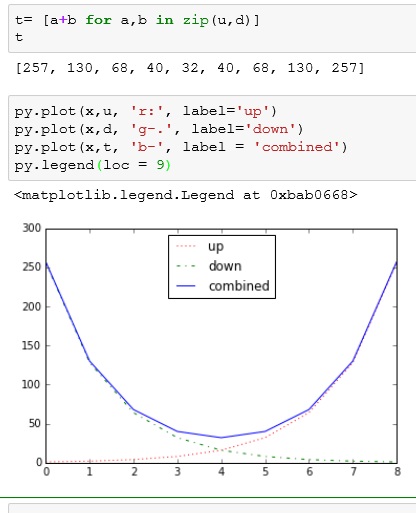
Here I use another list comprehension  and zip to make our last like. This adds each element of list u and d in order.

  • ‘b-‘ – blue solid line

pythonLine6


If you enjoyed this lesson, click LIKE below, or even better, leave me a COMMENT. 

Follow this link for more Python content: Python