Python Web Scraping: Using Selenium to automate web

This is follow up to how to connect to Chrome using Selenium. If you do not know how to get to a website on Chrome using Selenium, go here

To refresh. here is the code we used to open up a web page (in this case Wikipedia’s home page)

If you run this code, you should find yourself on the home page for Wikipedia

Okay, so now lets learn how to interact with page, the first thing I am going to do is to select the English language version of the page. There are a few ways go about this, but one of the easier approaches is to look at the HTML code that creates the page and to use xpaths or titles to find the object you are looking at.

Right click on the link for English and click inspect from the drop down.

If you get a body link first, you might need to right click and hit inspect again

To check if you have the right element, hover your mouse over it, and it will be highlighted on the webpage

Once you have the right element, right click on it, go to copy>Copy Xpath

Chose Xpath, not full Xpath, it makes for easier coding. You XPath should look something like this: //*[@id=”js-link-box-en”]/strong * When you go to try this, your XPath may look different. As websites are constantly updated, many of the Xpaths get updated as well. Go with the one you find when you Inspect the HTML code yourself

Now we are going to use selenium to “Find” the element we want. The code is dr.find_element_by_XPath(‘//*[@id=”js-link-box-en”]/strong’) *Note the use of single quote around the XPath, it is better to use them as many XPaths will contain double quotes

Once you have run that code, Selenium knows what element you are looking at, you can interact with it now. Let’s “click” the link

Note something i did in the code, I added a link= before my find element command. This assigned the element now to a variable. I can now use the “click()” method the variable inherited from the selenium.webdriver object to click on the English link

I could have just done this: dr.find_element_by_xpath(‘//*[@id=”js-link-box-en”]/strong’).click()

But by assigning the variable it is a) cleaner code and b) the link can be reused by my code later. Remember, it is a law of programming that you will always have to go back and fix something you haven’t seen in 6 months, so make the code as clean as possible to make future you less likely to develop a drinking problem due to having to fix poorly written code.

If you run the code above, you will move to the home English page

Lets try one more thing, lets typing a search into the search bar:

Right click > inspect the search bar, then right click>copy>copy xpath the selection in the HTML code

Now that you have the XPath, lets use the find_element_by_xpath code and a new command, send_keys() to input characters into the search box

Finally, right click on the magnifying glass>inspect>copy>copy Xpath and let us click on it to finish our search. (remember to hover over to make sure you have the right link)

Now you should find yourself on the Data Science page of Wikipedia

Now remember — the xpaths I have on this page will likely be out of date by the time you try this, so make sure to inspect the elements and get the correct XPaths for this work for you.

Python Web Scraping / Automation: Connecting to Chrome with Selenium

Selenium is a Python package that allows you to control web browsers through Python. In this tutorial (and the following tutorials), we will be connecting to Googles Chrome browser, Selenium does work with other browsers as well.

First you will need to download Selenium, you can use the following commands depending on your Python distribution

c:\> Pip install selenium

c:\> Conda install selenium

If you are on a work computer or dealing with a restrictive VPN, the offline install option may help you: Selenium_Install_Offline

Next you need to download the driver that let’s you manage Chrome through Python.

Start by determining what version of Chrome you have on your computer

Click on the three dots in the right corner of your Chrome browser, select Help> About Google Chrome

Go to https://chromedriver.chromium.org/downloads to download the file that matches your Chrome version. (note, this is something you will need to do every time Chrome is updated, so get used to it.)

Open up the zipfile you downloaded, you will find a file called chromedriver.exe

Put it somewhere you can find, put in the following code to let Python know where to find it.

from selenium import webdriver
options = webdriver.ChromeOptions()
options.add_argument("--start-maximized")
dr = webdriver.Chrome('C:/Users/larsobe/Desktop/chromedriver.exe',chrome_options=options)

Now to see if this works, use the following line, (you can try another website if you choose)   

Note the message Chrome is being controlled by automated test software.

You are now running a web browser via Python.

Python: Simulate Blockchain Mining

In my earlier tutorial, I demonstrated how to use the Python library hashlib to create a sha256 hash function. Now, using Python, I am going to demonstrate the principle of blockchain mining. Again using BitCoin as my model, I will be trying to find a nonce value that will result in a hash value below a predetermined target.

We will start by simply enumerating an integer through our sha 256 hash function until we find a hash with 4 leading zeros.

I used a while loop, passing the variable “y” through my hashing function each time the loop runs. I then inspect the first 4 digits [:4] of my hash value. If the first four digits equal 0000 then I exit the loop by setting the found variable to 1

(*note, a hash value is a string – hence the need for quotes around ‘0000’)

2018-04-27_13-30-18

As you can see in the version above, it took 88445 iterations to find an acceptable hash value

Now, using the basic example of a blockchain I gave in an earlier lesson, let’s simulate mining a block

2018-04-04_12-39-34

You’ll see, I am now combining the block number, nonce, data, and previous hash of my simulated block and passing it through my encryption function.  Just like in BitCoin, the only value I change per iteration is the Nonce. I keep passing my block through the hashing function until I find the Nonce that gives me a hash below the target.

2018-04-27_13-36-38

Now, let’s lower the target value to 6 leading zeros. This should result in a longer runtime to get your hash

2018-04-27_13-37-16

To measure the run time difference, let’s add some time stamps to our code

2018-04-27_13-39-31.png

So, I am using the timestamp function twice. D1 will be our start time, d2 will be our end time, and I am subtracting d1 from d2 to get our elapsed time. In the example below, my elapsed time was 5 secs

2018-04-27_13-50-43

Now, let’s bump the target down to 7 leading zeros. Now this brings my elapsed computing time to 20 minutes. That is a considerable commitment of resources. You can see why they call it a “proof of work” now.

2018-04-27_14-26-04


Python: Create a Blockchain Hash Function

If you are at all like me, reading about a concept is one thing. Actually practicing it though, that helps me to actually understand it. If you have been reading my blockchain tutorial, or if you came from an outside tutorial, then you have undoubtedly read enough about cryptographic hashes.

Enough reading, let’s make one:

( if you are unfamiliar with crytographic hashes, you can reference my tutorial on them here: Blockchain: Cryptographic Hash )

For this example, I am using the Anaconda Python 3 distribution.

Like most things in Python, creating a hash is as simple as importing a library someone has already created for us. In this case, that library is: hashlib

So our first step is to import hashlib

import hashlib

Now let us take a moment to learn the syntax require to create a cryptographic hash with hashlib. In this example, I am using the SHA 256 hashing algorithm. I am using this because it is the same algorithm used by BitCoin.

Here is the syntax used

hashlib.sha256(string.encode()).hexdigest()

To understand the syntax, we are calling the hashlib method sha256(): hashlib.sha256()

Inside the brackets, we are entering the string we want to encode in the hash. Yes it must be a string for this function to work.

Still inside the brackets we use the method .encode() to (surprise, surprise) ENCODE the string as a hash

Finally, I added the method .hexdigest() to have the algorithm return our hash in hexadecimal format. This format will help in understanding future lessons on blockchain mining.

So in the example below, you can see that I assigned the variable x the string ‘doggy’. I then passed x to our hash function. The output can be seen below.

2018-04-19_15-52-05.png

Now a hash can hold much more than just a simple word. Below, I have passed the Gettysburg Address to the hashing function.

(**note the ”’ ”’ triple quotes. Those are used in Python if your string takes up more than one line **)

2018-04-19_15-54-59

Now I try passing a number. You will notice I get an error.

2018-04-19_15-55-41.png

To avoid the error, I turn the integer 8 into a string with the str() function

2018-04-19_15-56-17.png

Below I concatenation a string and an integer.

2018-04-19_15-57-13.png

Last I want to show the avalanche effect of the hash function.

2018-04-19_15-58-01

By simply changing the first letter from an uppercase T to a lowercase t the hash changes completely. This is a requirement for hashing functions. If the hash did not change dramatically from a small change to the string, it would be easy to reverse engineer the hash. This is known as the avalanche effect.

2018-04-19_15-58-27


Python: An Interesting Problem with Pandas

I was writing a little tongue and cheek article for LinkedIn on fraud detection using frequency distributions (you can read the article here: LinkedIn). While this was a non-technical article, I wanted to use some histograms from a real data set, so I uploaded a spread sheet into Python and went to work.

While working with the data I ran into an interesting problem that had me chasing my tail for about 10 minutes before I figured it out. It is a fun little problem involving Series and Dataframes.

As always, you can upload the data set here: FraudCheck1

Upload the data.

import pandas as pd
df = pd.read_excel
("C:\\Users\\Benjamin\\OneDrive\\Documents\\article\\python\\FraudCheck1.xlsx")
df.head()

pandasProb.jpg

The data is pretty simple here. We are concerned with our answer column and the CreatedBy (which is the employee ID).  What I am trying to do is see if the “answer”  (a reading from an electric meter) are really random or if they have been contrived by someone trying to fake the data.

First, I want to get the readings for all the employees, so I used pop() to place the answer column into a separate list.

df1 = df

y = df1.pop("answer")

pandasProb1.jpg

Then, to make my histogram more pleasant looking, I decided to only use the last digit before the decimal. That way I will have 10 bars (0-9). (Remember, this is solely for making charts for an article. So I was not concerned with any more stringent methods of normalization)

What I am doing below is int(199.7%10). Remember % is the modulus – leaves you with the remainder and int converts your float to an integers. So 199.7 is cut to 199. The 199/10 remainder = 9.

a= []
i = 0 
while i < len(y):
     a.append(int(y[i]%10))
     i += 1
a[1:10]

pandasProb2

Then I created my histogram.

%matplotlib inline
from matplotlib import pyplot as plt
plt.hist(a)

pandasProb3.jpg

Now my problem

Now I want graph only the answers from employee 619, so first I filter out all rows but the ones for employee 619.

df2 = df.query('CreatedBy == 619')
y1 =df2.pop("answer")

Then I ran my loop to turn my answers into a single digit.

And I get an error.  Why?

pandasProb4.jpg

Well the answer lies in the datatypes we are working with. Pandas read_excel function creates a Dataframe.

When you pop a column from a dataframe, you end up with a Series. And remember a series is an indexed listing of values.

Let’s look at our Series. Check out the point my line is pointing to below. Notice how my index jumps from 31 to 62. My while loop counts by 1, so after 31, I went looking for y1[32] and it doesn’t exist.

pandasProb5.jpg

Using .tolist() converts our Series to a list and now our while loop works.

pandasProb6.jpg

And now we can build another histogram.

pandasProb7.jpg

The Code

import pandas as pd
df = pd.read_excel
("C:\\Users\\Benjamin\\OneDrive\\Documents\\article\\python\\FraudCheck1.xlsx")
df.head()

df1 = df
y =df1.pop("answer")

a= []
i = 0 
while i < len(y):
   a.append(int(y[i]%10))
   i += 1
a[1:10]

%matplotlib inline
from matplotlib import pyplot as plta1 = []
i = 0
while i < len(y2):
 a1.append(int(y2[i])%10)
 i = i+1
a1[1:10]

plt.hist(a)

df2 = df.query('CreatedBy == 619')
y1 =df2.pop("answer")

y2= y1.tolist()
type(y2)

a1 = []
i = 0
while i < len(y2):
    a1.append(int(y2[i])%10)
    i = i+1
a1[1:10]

plt.hist(a1)


Python: Naive Bayes’

Naive Bayes’ is a supervised machine learning classification algorithm based off of Bayes’ Theorem. If you don’t remember Bayes’ Theorem, here it is:

bayes

Seriously though, if you need a refresher, I have a lesson on it here: Bayes’ Theorem

The naive part comes from the idea that the probability of each column is computed alone. They are “naive” to what the other columns contain.

You can download the data file here: logi2

Import the Data

import pandas as pd
df = pd.read_excel("C:\Users\Benjamin\Documents\logi2.xlsx")
df.head()

nb.jpg

Let’s look at the data. We have 3 columns – Score, ExtraCir, Accepted. These represent:

  • Score – Student Test Score
  • ExtraCir – Was Student in an Extra Circular Activity
  • Accepted – Was the Student Accepted

Now the Accepted column is our result column – or the column we are trying to predict. Having a result in your data set makes this a supervised machine learning algorithm.

Split the Data

Next split the data into input(score and extracir) and results (accepted).

y = df.pop('Accepted')
X = df

y.head()

X.head()

nb1.jpg

Fit Naive Bayes

Lucky for us, scikitlearn has a bit in Naive Bayes algorithm – (MultinomialNB)

Import MultinomialNB and fit our split columns to it (X,y)

from sklearn.naive_bayes import MultinomialNB
classifier = MultinomialNB()
classifier.fit(X,y)

nb2.jpg

Run the some predictions

Let’s run the predictions below. The results show 1 (Accepted) 0 (Not Accepted)

#--score of 1200, ExtraCir = 1
print(classifier.predict([1200,1]))

#--score of 1000, ExtraCir = 0
print(classifier.predict([1000,0]))

nb3

The Code

import pandas as pd
df = pd.read_excel("C:\Users\Benjamin\Documents\logi2.xlsx")
df.head()

y = df.pop('Accepted')
X = df

y.head()
X.head()

from sklearn.naive_bayes import MultinomialNB
classifier = MultinomialNB()
classifier.fit(X,y)

#--score of 1200, ExtraCir = 1
print(classifier.predict([1200,1]))

#--score of 1000, ExtraCir = 0
print(classifier.predict([1000,0]))


Python: K Means Cluster

K Means Cluster will be our introduction to Unsupervised Machine Learning. What is Unsupervised Machine Learning exactly? Well, the simplest explanation I can offer is that unlike supervised where our data set contains a result, unsupervised does not.

Think of a simple regression where I have the square footage and selling prices (result) of 100 houses. Taking that data, I can easily create a prediction model that will predict the selling price of a house based off of square footage. – This is supervised machine learning

Now, take a data set containing 100 houses with the following data: square footage, house style, garage/no garage, but no selling price. We can’t create a prediction model since we have no knowledge of prices, but we can group the houses together based on commonalities. These groupings (clusters) can be used to gain knowledge of your data set.

I think seeing it in action will help.

If you want to play along, download the data set here: KMeans1

The data set contains a 1 year repair history of 197 Ultrasound medical devices.

Data dictionary (ID Tag – asset number assigned device, Model – model name of device, WO Count – count of repair work orders, AVG Labor – average labor minutes per repair, Labor Cost – average labor cost per repair, No Problem-  count of repairs where no problem was found, Avg Cost -average cost of parts, Travel – average travel hours per repair, Travel Cost – average travel cost per repair, Department – department that owns the ultrasound device)

kmeans

We want to see what kind of information we can extract from this data.

To do so, we are going to use K Means Clustering.

How does K Means Clustering work? Each row in the table is converted to a vector. Imagine the vectors now graphed in N-dimension space. Next pick the number of clusters you want to create. For each cluster, you will place a  point(a centroid) in space and the vectors are grouped based on their proximity to their nearest centroid.

The calculation to tell proximity is made using geometric means (not arithmetic)- hence the name K-Means Cluster

(each dot below is a row in your table, the colors represent a cluster)

kmeans2

Let’s do it in Python

Import the data.

import pandas as pd

df = pd.read_excel("C:\Users\Benjamin\Documents\KMeans1.xlsx")
df.head()

kmeans1

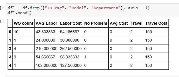
Now, we are going to drop a few columns: ID Tag – is a random number, has no value in clustering. Then Model and Department,as they are text and while there are ways to work with the text, it is more complicated so for now, we are just going to drop the columns

df1 = df.drop(["ID Tag", "Model", "Department"], axis = 1)
df1.head()

kmeans2

Now lets import KMeans from sklearn.cluster

We then initialize KMeans (n_clusters= 4 -no of clusters you want, init=’k-means++’ -sets how the centroids are places. k-means++ is one of the faster methods of centroid placement, n_init=10 – number times the algorithm with run placing new centroids each iteration)

from sklearn.cluster import KMeans
km = KMeans(n_clusters=4, init='k-means++', n_init=10)

kmeans3.jpg

Choosing number of clusters is a bit of an art. Play with it a bit and see how different values play out for you.

Now fit the model

km.fit(df1)

kmeans4.jpg

Now, export the cluster identifiers to a list. Notice my values are 0 -3. One value for each cluster.

x = km.fit_predict(df1)
x

kmeans5.jpg

Create a new column on the original dataframe called Cluster and place your results (x) in that column

df["Cluster"]= x
df.head()

kmeans6.jpg

Sort your dataframe by cluster

df1 = df.sort(['Cluster'])
df1

kmeans7.jpg

Now as you start to examine the data in each cluster, you show start to see patterns emerge.

Below is an example of the patterns I found in the clusters.

kmeans9.jpg

Now remember, this is just an INTRODUCTION to unsupervised learning. We will learn more tricks to help you discover the patterns as we move forward.

Python: K Nearest Neighbor

K Nearest Neighbor (Knn) is a classification algorithm. It falls under the category of supervised machine learning. It is supervised machine learning because the data set we are using to “train” with contains results (outcomes). It is easier to show you what I mean.

Here is our training set: logi

Let’s import our set into Python

knn.jpg

This data set contains 42 student test score (Score) and whether or not they were accepted (Accepted) in a college program.  It is the presence of the Accepted column that makes supervised machine learning possible. Knowing the outcomes of past events, we can create a prediction model for future events. So you could use the finished model to predict whether someone will be accepted based on their test score.

So how does Knn work?

Look at the chart below. Imagine this represents our data set. Each blue dot is accepted (1) while each red dot is not(0).

knn1

What if I want to know about my new data point (green star)? Is it a 1 or a 0?

knn2

I start by choosing a neighbor count – in this example I will choose 3, and I find the 3 nearest neighbors to my new point.

Let’s look at the results, I have 2 red(0) and 1 blue(1). Using basic probability, I am 67% (2/3) certain that you will not get in.

knn3.jpg

Now, let’s code it!

First we need to separate our data into 2 dataframes: Our training set X (Score) and our target set y (Accepted)

df.pop() removes the Accepted column from your dataframe and places it in a newly created one.

knn4.jpg

knn5.jpg

Import sklearn

sklearn is a massive library of machine learning algorithms available for Python. Today we are going to use KNeighborsClassfier

So below imported KNeighborsClassifier from sklearn.neighbors

Next I set my neighbor count to 5. You can experiment with other numbers and see how works out for you. Setting the neighbor count is something you kind of have to develop a feel for.

knn6.jpg

Now let’s fit the model with our training set(X) and target set(y)

knn7

Now we can use our model to make predictions.

ne.predict() will return 1 or 0 – (Accepted or Not)

while ne.predict_proba() will return a probability range. Results below read as (40% change of not Accepted(0), 60% chance of Accepted(1))

knn8.jpg

So there you go, you have now built a prediction model using K Nearest Neighbor.


Python: Logistic Regression

This lesson will focus more on performing a Logistic Regression in Python. If you are unfamiliar with Logistic Regression, check out my earlier lesson: Logistic Regression with Gretl

If you would like to follow along, please download the exercise file here: logi2

Import the Data

You should be good at this by now, use Pandas .read_excel().

df.head() gives us a the first 5 rows.

What we have here is a list of students applying to a school. They have a Score that runs from 0 -1600,  ExtraCir (extracurricular activity) 0 = no 1 = yes, and finally Accepted 0 = no 1 = yes

logi1

Create Boolean Result

We are going to create a True/False column for our dataframe.

What I did was:

  • df[‘Accept’]   — create a new column named Accept
  • df[‘Accepted’]==1  — if my Accepted column is 1 then True, else False

logi1

What are we modeling?

The goal of our model is going to be to predict and output – whether or not someone gets Accepted based on some input – Score, ExtraCir.

So we feed our model 2 input (independent)  variables and 1 result (dependent) variable. The model then gives us coefficients. We place these coefficients(c,c1,c2) in the following formula.

y = c + c1*Score + c2*ExtraCir

Note the first c in our equation is by itself. If you think back to the basic linear equation (y= mx +b), the first c is b or the y intercept. The Python package we are going to be using to find our coefficients requires us to have a place holder for our y intercept. So, let’s do that real quick.

logi2


Let’s build our model

Let’s import statsmodels.api

From statsmodels we will use the Logit function. First giving it the dependent variable (result) and then our independent variables.

After we perform the Logit, we will perform a fit()

logi3.jpg

The summary() function gives us a nice chart of our results

logi4.jpg

If you are a stats person, you can appreciate this. But for what we need, let us focus on our coef.

logi45.jpg

remember our formula from above: y = c + c1*Score + c2*ExtraCir

Let’s build a function that solves for it.

Now let us see how a student with a Score of 1125 and a ExCir of 1 would fair.

logi9

okayyyyyy. So does 3.7089 mean they got in?????

Let’s take a quick second to think about the term logistic. What does it bring to mind?

Logarithms!!!

Okay, but our results equation was linear — y = c+ c1*Score + c2*ExCir

So what do we do.

So we need to remember y is a function of probability.

logis1

So to convert y our into a probability, we use the following equation

logis2

So let’s import numpy so we can make use of e (exp() in Python)

logi8.jpg

Run our results through the equation. We get .97. So we are predicting a 97% chance of acceptance.

logi10.jpg

Now notice what happens if I drop the test score down to 75. We end up with only a 45% chance of acceptance.

logi11.jpg


If you enjoyed this lesson, click LIKE below, or even better, leave me a COMMENT. 

Follow this link for more Python content: Python


Python: Accessing a SQL database

create database sandbox;

use sandbox;
CREATE TABLE employee_id (
        emp_nm varchar(30) not null,
        emp_id varchar(8),
        b_emp_id varchar(8),
        PRIMARY KEY(emp_nm) );   

If you really want to do data work, you need to be able to connect to a database. In this example I will show you how to connect to and query data from MS SQL Server with the AdventureWorks2012 database installed.

This lesson assumes some very basic knowledge of SQL. If SQL is a complete mystery, head over to my SQL page: SQL  If you check out the first 4 intro lessons, you will know everything about SQL you need to know for this lesson.

Install pyodbc

To connect to the database, we need to install pyodbc. Go to your Anaconda terminal and type: pip install pyodbc

sqlpython.jpg

Now open up your jupyter notebook and start a new notebook

Connect to Database

import pyodbc

cnxn is our variable – it is commonly used as a shorten version of connection

syntax: pyodbc.connect(‘DRIVER={SQL Server}; SERVER=server name; DATABASE=database name;UID = user name; PWD = password’)

finally cursor =cnxn.cursor() creates a cursor for us. In SQL, a cursor is used to step through your results one row at a time.

sqlpython1.jpg

cursor.execute(place sql query here)  – this is how you pass a sql query – note query goes in quotes

tables = cursor.fetchall() – fetch all the rows in your query results

sqlpython2

We can now iterate through the rows in tables.

sqlpython3.jpg

I don’t like the layout of this. Also we can’t really work with the data.

Pandas Dataframe

first import pandas

  • d= [] – create empty dictionary
  • d.dappend({‘Name’:row.Name, ‘Class’: row.GroupName}) – fill dictionary 1 row at a time
  • df = pd.DataFrame(d) – convert your dictionary to a dataframe

sqlpython4.jpg


If you enjoyed this lesson, click LIKE below, or even better, leave me a COMMENT. 

Follow this link for more Python content: Python