Linear Regression using Excel

Link to video on Linear Regression using Excel

Regression Analysis is still the most popular method used in Predictive Analytics. The main reason is that it works. It is well known and understood. With its different flavors, regression analysis covers a width swath of problems. Another great reason to use it, is that regression tools are easy to find.

Today we are going to use Excel to tackle a simple regression problem. I have uploaded a spreadsheet to this page. If you would like to follow along with the exercise, please download it from the link below:

Excel File Download:  Linear Regression Example File 1

What is Linear Regression?

Linear Regression is a method of statistical modeling where the value of a dependent variable based can be found calculated based on the value of one or more independent variables. The general idea, as seen in the picture below, is finding a line of best fit through the data. Using that line, you can then predict the value of Y given X.

linear1

I am not going to go too deep into the math here. I highly the Khan Academy video posted below if you are looking to brush up on your statistics.

Khan Academy – Linear Regression

Lets Start by Looking at the Data

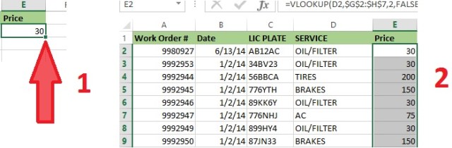
If you download the Excel file at the top of the page, you will find 2 columns labeled Years and Salary. This example data set shows us the years of service and salary of 39 employees for an imaginary company.

linear2

What we are going to attempt to do is to develop a model using Linear Regression that will allow us to predict the salary of an employee given their years of service.

Step 1: Build a Scatter Plot

The first thing we want to do is build a scatter plot. Excel makes this simple enough. Just highlight all of your data > select the Insert Tab from the Ribbon > Select Scatter from Charts:

linear3.jpg

What you will get should look something like this:

linear4

We have a scatter chart with Salary on the Y Axis and Years on the X Axis. **Excel scatter charts set the left most column of the data set to the X Axis by default.

Before we move on, I want to take a moment to look at the scatter plot. Do you see a pattern? Can you see where you might be able to draw a line through the data?

I am not trying to just fill space here. I am asking a serious question. Because the answer is sometimes you will not see a pattern. Sometimes the scattering of data will be so random that there will no need to go forward with a linear regression. Learning to look for patterns in data visualizations is skill worth developing.

linear5

In this example there is a general pattern, or more accurately, we see what looks like Positive Correlation. We call it positive because it appears that as X increases so does Y. So now that our scatter chart has passed the visual test, it is time perform our regression.

Trend Line

Performing a simple linear regression in Excel is ridiculously easy. Simply click on your scatter plot > from the Ribbon select Chart Tools – Design > Add Chart Element > Trendline > Linear

linear6.jpg

Your trendline appears on your chart. I personally find the line a little hard to see as is, so I am going to format it a bit.

linear7

Start by double clicking on the trendline and the Format Trendline window will open on the right.

I made the following changes:

Line: — Color: Red  — Width: 3pt  — Dash type: Solid Line

Trendline Options — Select Display Equation on chart and Display R-squared value on chart

linear8

Alright, that line is much easier to read. Now let us talk about the numbers in the circle. Now I know I said I was not going to get too deep into the math, but I feel I can’t do this subject justice without at least a cursory explanation of what is going on.

linear9

What exactly did Excel do when it added the trendline? Technically it performed a statistical function known as Ordinary Least Squares.  What does that mean? Well if you wanted to attempt this by hand, one approach you could take would be to start by drawing a line that looked best to you. You would then measure the Residuals (the distance from the actual data points and line you drew)

linear10

You then repeat the process (picking a new line and measuring residuals) until you find the line that results in the lowest overall residual.Once you have it, you get the equation for your line:  y = 1357.9x+50974 (Luckily for us Excel makes the process a lot easier)

Now a quick refresher on the line formula: Y= mX + b (where m = Slope and b = Y-Intercept). This equation is what you would use to make predictions. In our equation a person with 0 years in service would have a salary of 50974: Y = 1357.9(0) + 50974 — Y= 50974. And each year of service would add 1357.90 to the salary.

Before we go start using your equation to start making predictions, we still need to discuss the R² you see below your line equation. I won’t bore you with how R² is calculated. You don’t really need to know how it is calculated to use linear regression, but you do need to know how to read it.

The simplest explanation I can give you for R² is that a value of 1 means perfect fit – every point in your data matches up to your line. 0 on the other hand, means your line doesn’t match anything. Our R² is 0.4423, which really is not that great. I generally prefer to aim for a R² value above 0.6.

How can we improve our R² value? My preference would be to get more data. We currently only have 39 tuples. More data could improve our accuracy. If more data is not available though, you can look at your outliers as Linear Regression can be greatly affected by outliers. Unfortunately outliers are often tricky to deal with. A person with 1 year of service making 100,000 a year would definitely be an outlier, but it is not an impossibility. If this employee is a highly experienced individual who just transferred from another company, it is totally feasible they could be earning 100,000.

The hard truth is, considering only the data we have, we cannot rightfully develop a reliable model. This happens more often than you might think. That is okay though, we will chalk this up as a learning experience and move on.


Analytics: An Introduction

So exactly what is Analytics? Everyone is talking about it. Colleges and Universities are scrambling to develop programs in it. But what exactly does it mean?

Definition

The the definition I like the best is this:

Analytics: Discovering and communicating meaningful patterns in data.

Analytics are traditionally broken down into the following catagories:

  • Descriptive Analytics: Most people are familiar with this form. So familiar in fact, they probably do not refer to it as analytics. This is looking at past and current data to describe what is going on. Most standard business reporting falls into this category.
  • Predictive Analytics: This is using available data to help predict future events or to provide best guess answers to fill in gaps in data. Using predictive analytics, you can predict how much a house will sell for or what items you should stock near the registers based on current conditions (example: Walmart discovered Pop-Tarts tend to sell well during hurricanes).
  • Prescriptive Analytics: This is the cutting edge of analytics. Prescriptive analytics not only makes predictions about future events, but it utilizes decision making algorithms to determine how to respond to the events. Prescriptive analytics engines could, using the Pop Tarts example above, automatically reroute the shipment of Pop Tarts to stores in hurricane affected areas without any human intervention.

It should be noted that most companies today are still spending most of their time in the descriptive analytics world. That is not necessarily a bad thing. Being able to get the right information in front of a decision maker, in a format that is easily digestible, is a talent all within itself. 

Components

Analytics is not a 1 step process. It is actually a series of steps, often performed in an iterative manner. And just as each business problem is unique, so are the steps to the analytics process used to find the solution.

While the statement above is 100% percent true, I find it very unsatisfying. This is the kind of information I would find when I first developed an interest in analytics. So while I cannot give you a one size fits all answer, I feel that I at least owe you a better explanation than that.

For me, perhaps the best way to understand analytics, is to look at some of the more common tasks performed.

  • Data Management: While designing, building, and maintaining databases and data warehouses may not typically fall under the responsibility of an analytics professional, having a general understanding of how they work is none the less important. Databases and data warehouses are where most businesses keep their data. If you want to be taken seriously as a data professional, you need to have a fundamental understanding of how data is stored and how to query the stored data. (Example Technologies: Hadoop, SQL Server, Oracle)
  • Data Modeling: Data modeling is organizing data into logical structures so that is can be understood and manipulated by a machine. As a simple exercise, make a quick spreadsheet for sales amounts for  5 salespeople across 4 quarters. When you are done, look at the table you created. You have just modeled data. (Example Technologies: Excel, SQL Server, Oracle, Visio)
  • Data Cleaning: While this may not be the sexiest part of the job, it is the part you will spend the most time on. 60-80% of your time will be spent in this phase of the job. And while there are some third party software applications out there that can help ease the pain (Alteryx comes immediately to mind), they are expensive and not every boss will be willing to spring for it. My suggestion is to put sometime aside to become very familiar with Excel. I do 90% of my data cleaning work in Excel and MS SQL Server. (Example Technologies: Excel, SQL Server, Oracle, Alteryx)
  • Data Mining (Machine Learning): Now this is the cool stuff everyone is talking about. Data mining or machine learning, whichever you prefer to call it,  is the Artificial Intelligence (AI) portion of analytics. Data mining is difficult to provide a simple explanation for, but I will try anyway: In traditional programming, the programmer provides explicit instructions to the computer as to how to perform a task. With data mining, data sets are fed through an algorithm. The computer then determines the best way to solve the problem based on the data provided. 

 To help make this a little clearer, how about you try your hand at being the machine.

spam

Look at the pattern above. Without me providing you with any more information,                  you should be able to determine, that two blue squares in a row = SPAM. This is, at                 the most fundamental level, how data mining works. It pours over data and finds                   patterns. Knowing this pattern, if you were now shown only the first three columns               you would be able to predict whether the last column would be red or green.(Example Technologies: R, Python, SAS, XLMiner)

  • Data Visualization: DataViz is fun. It is the real show stopper in the data world. Visualizations make the patterns pop off the page. There are a lot of great programs out there for data visualization. (Again, do not discount Excel — it has some great DataViz features). Now DataViz should rightfully be broken into two separate categories. The first is Exploratory. This is visualizations used by the data professional to help analyze and understand the data. The second is Production. This the finished product that ends up on reports and dashboards for the business users to see. (Example Technologies: Excel, Tableau, R, SAS)
  • Optimization and Simulation: How often is there truly only one solution for a problem? Reality is sometimes the hardest part isn’t coming up with a solution to a problem, but deciding which solution to use. Building optimization models and running simulations helps to provide decision makers with quantitative data as to which solutions will be most effective. (Example Technologies: CPLEX, SAS, Solver)

So I have to learn all of this…

That depends – If your goal to is be a Data Scientist, then yes, you need to learn everything mentioned above and then some (I hope you love Statistics). However, if you are a business user just trying to add analytic skill to your toolbox, my recommendation is to focus your efforts on becoming efficient in data cleaning. In the real world, when trying to put a report together, you often are given data from multiple sources and you have to cobble it together to make sense of it. Learning some data cleaning skills can save you hours on tasks like that.

Once you have workable data, take some time to learn some visualization techniques. An eye popping chart will always garner more attention than pages of numeric columns. Also, take a little time to learn some data mining skills. No one is expecting you to write the complex algorithms the PhD’s at Stanford and MIT are kicking out, but there actually are some pretty user friendly data mining programs out there that help you cull some real insight out of your data.

However you decide to go about it, Analytics is a fascinating, fast growing field. It truly is a 21st century skill. Here at Analytics4All.org, the philosophy is that everyone should develop some analytical talent. Computers were once the sole territory of the science geeks of the world and now they are in everyone’s pockets and purses. Analytics and data driven decision making should also be a accessible to all.

Excel: Learning to Use Formulas

The first step towards being an Excel Power User is learning to use formulas. Pulling out a calculator to add up Excel columns is a sure fire way to let everyone in the office know your computer skills are lacking. Luckily for you, basic Excel formulas are pretty easy learn.

Lesson 1: Basic Arithmetic Formulas

Video Link: Excel Formulas Part 1

Excel supports all standard Arithmetic functions – addition, subtraction, multiplication, division, etc. **Excel comes standard with advanced engineering and statistical functions, but that is well beyond the scope of this article.

To start a formula in Excel: select the cell where the result belongs and type =. Using = as the first character tells Excel you want to create a formula.

In this example, we want to add the first row of column A and B and place the answer in C. Select cell C2, enter =A2+B2. Press enter and 7 will appear in the space. Try changing the values in cells A2 and B2. Notice the value in C2 changes in kind.

formulas1

Notice how as you type in a formula, it populates in the formula bar above as well. You can work in the formula bar instead if you chose (as your formulas get longer and more complex, you will find yourself doing more work in the formula bar).

You can try out some other arithmetic functions following the example below: **note: make sure to start your formulas with =

formula2

Lesson 2: Replicating Formulas

Video Link: Excel Formulas Part 2

If you had to input each formula individually every time you wanted to use one, this would not be any more efficient then simply doing the calculations on your old desktop calculator. Fortunately, Excel makes replicating your formulas across many cells as simple as clicking a mouse button.

In the bottom right corner of an active cell, there is a small green box. You can click on this box and drag it over the cells you would like the formula to replicate. Or, you can just double click corner and it will automatically replicate the remaining rows in your table.

formula3

Lesson 3: Functions

Video Link: Excel Part 3

Excel has hundreds of built in functions (far too many to cover in this article). These functions save you having to write complex formulas manually.

Below are examples of 3 commonly used functions (SUM, PRODUCT, AVERAGE)formula4

Let us break these functions down:

  1. SUM() — adds the values of all cells listed in the parenthesis.  **In the example above, the SUM function has C2:C5 in the parenthesis. The colon(:) means between. So C2:C5 actually means all the values C2 through and including C5 (C2,C3,C4,C5)
  2. PRODUCT() — multiplies the values of all cells listed in the parenthesis.
  3. AVERAGE() — takes the average of the values of all cells listed in the parenthesis.

If you are curious as to what other built in functions Excel offers, go to the Formulas tab in the ribbon cable. 

formula6


Numbers don’t add up in Excel

With the popularity of Excel, it is no wonder many third party applications offer a feature to allow you to export data directly into Excel. This is convenient and makes it easy to share information as almost everyone has Excel loaded on their computer. Unfortunately, often these files (due to poor coding from the third party application) do not have full functionality.

The Problem: Numeric Columns Don’t Add Up

Your boss receives a file from your purchasing department. It is a monthly breakdown parts expenditures for your maintenance department. The problem is, when he tries performing some basic arithmetic functions on the spreadsheet, the numbers don’t add up(literally). **Note the SUM() function in the picture below returns $0.00 even though there are positive values in the column above.

numbers


After attempting all the solutions he could think of, your boss sends the file to you hoping you can help him out.

The Solution: Hidden Characters

 After receiving the file, you discover the cause of the problem is hidden characters. Whatever application this spreadsheet was exported with, added a few hidden gems to make sure the file is utterly useless to anyone trying do much more than just read the file. 

So how do we fix the issue? First you will need a keyboard with a numeric keypad. Time to start digging through your desk drawers or making nice with the office hoarder. I am sure he has a few dozen keyboards squirreled away somewhere and can loan you one. Although it will probably be up to you to dust off the doughnut powder.

Okay, so you have your keyboard. Now what?

  1. Highlight cells you want to work with
  2. Go to Find&Select > Replace in the upper right corner of your ribbon bar

hidden1

3. In the Find what: field – hold down the ALT key and type 0160 with the numeric keypad. ***note nothing will appear in the space as you type this

4. Leave Replace with: blank and hit the Replace All radio button

Now all of your numeric columns will function properly.You can send the file back to your boss, further cementing your reputation as the office Excel guru.


Extract Date from DateTime in Excel

Have you ever exported an Excel file from a program and the formatting was all off? Even worse, when you try to fix the formatting, Excel won’t let you. One of the most common problems I run up against is date time formatting issues when I am dealing with Excel file that originated somewhere else.

The Problem: Date Time Format cannot be Changed

datechange

Here we have an Excel file in which one of the columns contains a date time stamp. The problem is, we do not care about the time, we only want the date. No matter what we do though, we can not seem to alter the date format.

None of the standard fixes help here. Formatting the cells, copying cells to a new sheet, and even using Special Paste results in a date time stamp we still cannot alter.

The Solution: Text to Columns

First things first – Make sure to select the date column in question.

datechange1

From the Ribbon Bar, go to the Data tab. You will see an Icon labeled Text to Columns.

datechange2

We are going to use Fixed width as the elements in the date time column all maintain a fixed size.

Hit next. Excel will place bars in the data preview window to show you how the data will be segmented. **Notice Date, Time, and AM/PM each occupy a separate column now.

datechange3

Since everything looks good, we will hit next.

Now highlight the date column, select Date from the Column data format box and chose your preferred date format from the drop down menu.

datechange4

For the next two columns, since we do not not need them in this example, we will just highlight each column and select Do not import column (skip)

datechange5

Now hit Finish and here are the results.

datechange7


Merging Data with Excel

Before you can do anything with your data, it has to be cleaned and prepped. While certain fixes (spelling errors, date format, number format, etc.) are easy enough to handle, merging multiple tables or worksheets together can be frustrating. I have witnessed seasoned Excel users reduced to manually inputting hundreds of data fields into their spreadsheet. If only they knew how to use the look up functions built into Excel.

Vlookup

Vlookup (and its transposed partner Hlookup) are 2 of the most common look up functions in Excel. And while they may seem complex at first, they are actually pretty easy to use.

Enough talk though, let us see how it works:

vlook1

Here are two tables from an imaginary auto repair shop. The Green Table shows a list of work orders, while the Yellow Table shows a pricing list for the services the shop offers.  So, the task at hand is to use the Yellow Table to populate a price column on the Green Table.

Start simply enough, go to the last column of the Green Table Right Click > Insert Column. Name the column Price and go to the first open cell in the column and input the following formula: =VLOOKUP(D2,$G$2:$H$&,2,FALSE)

vlook2

Now I know this looks complicated, but I promise it is not as bad as it looks.

  1. Start with =VLOOKUP()   **Whenever = is the first character in a cell, Excel automatically knows what follows is a formula.
  2. The first element inside the parenthesis of a VLOOKUP is the reference cell in your main table. In the example above, I chose cell D2 (seen in blue), which holds the service information for the first work order. This is the data field I want to reference against my lookup table.
  3. The next element is the range of the lookup table (seen in red). The lookup table range in this example is G2:H7. **After highlighting the lookup table, select F4 to lock the range in $G$2:$H$7. This ensures that as the VLOOKUP formula is replicated down the sheet,  the lookup table stays locked in place.
  4. The next element in the formula is the column that holds the return value. We are looking for the price from the Yellow Table, so column 2 holds the return value.
  5. The final element is Exact or Closest Match. FALSE means only exact matches. TRUE means closest matches.

Once the formula is complete, hit enter and the price will appear in the cell. Finally, replicate the formula down through all Work Order records in the Green Table.

vlook5

Excel tip: If you hover your mouse over the little green square the arrow is pointing to, your cursor will become a black plus sign. Double click on the green square and the formula will be replicated down all the remaining rows in your table.
vlook3