CPLEX: An introduction to Linear Programming with OPL

IBM’s CPLEX is a commercial quality Optimization product. It can handle 10’s of 1000’s of variables as well as massive data sets. As with most commercial software it is very expensive, but they do offer a limited edition you can download to get some experience working with it.

You can find the free downloads here: CPLEX Download

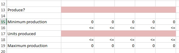
In this example, we will be using CPLEX OPL (optimization programming language) to solve a very simple linear problem. Check out the already solved solution below:

As you can see, we are deciding which of 2 types of furniture, Table and Chairs. Our goal is maximize our profit, however we only have 300 units of material and 110 units of labor available.

phpsimplex1

Let’s break it down into some basic formulas now.

First, what are the two main elements we have here? Furniture (Table, Chair) and Resources (Material and Labor). All other elements are related to either Furniture or Resources in some way.

How Many? is related to Furniture. To make this easier to follow we will shorten How Many? to HM

Profit per Unit is also related to furniture – let’s call it P

So Total Profit = HM[Table]*P[Table] + HM[Chair]+P[Chair]

In a bit more formal format: cplexFurn.jpg

Coding in CPLEX

Now let’s code this in CPLEX. First we need to create a new OPL Project

cplexFurn1.jpg

Name your project and make sure to check Create Model and Create Data

cplexFurn2.jpg

You will note you now have two new files, a .mod and .dat

  • .mod = model file
  • .dat = data file

cplexFurn3.jpg

We are going to start by building our model file.

The model file consists of 4 parts

  • Variable declaration
  • Decision variable declaration
  • Objective
  • Constraints

Variable Declaration

{string} furniture = ...;   
{string} resources = ...;
int P[furniture] = ...;
int Avail[resources] = ...;
int ResValue[resources][furniture] = ...;

First- the =…; means the variable will find its values in the .dat file. We will get there soon.

{string} furniture = …;   — blue box
{string} resources = …;  — red box

cplexFurn4.jpg

int P[furniture] = …;  – red box
int Avail[resources] = …;  –  green box
int ResValues[resources][furniture] = …;  – purple box

cplexFurn5

The [] after the variable name tells which string the variable is related to. If you having trouble seeing what I am talking about, look at the images below.

cplexFurn6.jpg

cplexFurn7

cplexFurn8.jpg

I know this is confusing, but hopefully it will clear up as we move forward.

Decision variable declaration

dvar int HM[furniture];

Our decision variable (dvar) is how many units to build (HM). This is of course related to furniture. As the picture below shows:

cplexFurn9.jpg

Objective:

maximize 
      sum(i in furniture)
                  HM[i]*P[i];

Our object is to maximize profit. The equation above is simply the OPL way of writing:

HM[Table]*P[Table] + HM[Chair]+P[Chair]

sum(i in furniture) is like a for loop where the results of each iteration are summed up. The two values passed through i would be Table and Chair.

Constraints:

subject to {

      forall(i in resources)
               ct1:
                   sum(j in furniture)
                         ResValue[i][j]*HM[j]<=Avail[i];

}

Our final chunk of code in our model (.mod) file is our Constraints. Constraints are started by using the code: subject to {}

Forall(i in resources) – is just a for loop iterating through (materials, labor)

ct1: – just names your constraint – an issue in bigger problems where you might have many constraints.

To clarify I will walk you through the sum(j in furniture) loop.

  1. ResValue[Materials][Table]*HM[Table]<=Avail[Materials]
  2. ResValue[Materials][Chair]*HM[Chair]<=Avail[Materials]
  3. ResValue[Labor][Table]*HM[Table]<=Avail[Labor]
  4. ResValue[Labor][Chair]*HM[Chair]<=Avail[Labor]

Here is what the code looks like in CPLEX

cplexFurn10.jpg

Now, let’s fill in our .dat (data file)

The code should be pretty self explanatory, note the use of {} for our string variables

furniture = {"Table","Chair"};
resources = {"Wood", "Labor"};
P = [6,8];
Avail = [300,110];
ResValue = [[30,20],[5,10]];

Here is the code in CPLEX

cplexFurn11.jpg

Run the code

To run the code, we first need to create a running configuration. Right click on Run Configurations > New > Run Configuration

cplexFurn12.jpg

Name your run configuration

cplexFurn13.jpg

Now, select you .mod and .dat files one at a time and drag them into your new running config. When you get the pop up warning, just click okay. Repeat this task for both files

cplexFurn14.jpg

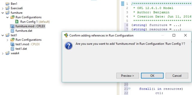
Here is what your screen should look like.

cplexFurn15.jpg

Right click your running config and click Run this

cplexFurn16.jpg

Click Okay to save your mod and dat file

cplexFurn17.jpg

And now we have our results. 96 is out total profit with 4 Tables and 9 Chairs being built. Just like our Solver solution above.

cplexFurn18.jpg

The Code

.mod file

{string} furniture = ...; 
{string} resources = ...;
int P[furniture] = ...;
int Avail[resources] = ...;
int ResValue[resources][furniture] = ...;

dvar int HM[furniture];

maximize 
 sum(i in furniture)
    P[i]*HM[i];
 
subject to {

forall(i in resources)
 ct1:
 sum(j in furniture)
 ResValue[i,j]*HM[j]<=Avail[i];

}

.dat file

furniture = {"Table","Chair"};
resources = {"Wood", "Labor"};
P = [6,8];
Avail = [300,110];
ResValue = [[30,20],[5,10]];


PHPSimplex: Simplex Linear Programming

So I received this message on Twitter early this morning. Always curious as to what else is out there, I went to the site and checked them out.

Link to website here: http://www.PHPSimplex.com/en/index.htm

phpsimplex.jpg

I will say I was pleased with what I found. This is actually a great way to cover the next topic I had in mind.

We have done a few Linear Programming models with Excel Solver already and I wanted to move on to show a bit more of the guts behind it. More advanced optimization tools don’t work off of spreadsheets, but instead require you to model your problem in a the form of a series of linear formulas.

Now if you check out the theory and examples section of the PHPSimplex website, they do have some good examples. But to better help you transition from spreadsheet to linear formulas, I am going to take an Excel Solver solution and show you how I would do it in PHPSimplex.

Below is a nice simple problem. We are building 2 types of furniture, tables and chairs. We are given the material and labor each item requires and the available amounts of each. We also have the profit per unit each item brings in. Our goal is to maximize profit. What we need to find out is how many of each item to build.

As you can see, this problem has already been solved using Excel Solver. Let’s see how we would approach this using PHPSimplex.

phpsimplex1.jpg

Go to the webite and click on the icon in the left corner or PHPSimplex in the menu bar.

phpsimplex2.jpg

I am going to select the Simplex/ Two Phases Method for this example

phpsimplex3.jpg

And based on our problem, I am going to choose 2 decision variables (my 2 pink changing cells) and two constraints (I will explain)

Now I am going to Maximize my function (I want max profits). Then I will set my function to 6X1+8X2 – The X1 and X2 represent my 2 changing cells. The 6 and 8 I get from my profit per unit found in my spread sheet.

So to put it in English : Max Profit = $6 * # of Tables Built + $8 * # of Chairs Built

phpsimplex5.jpg

Now our Constraints:

30X1 + 20X2 <= 300 – Materials – 30 * # Tables + 20 * # Chairs can’t exceed 300

5X1 + 10X2 <= 110 – Labor – 5 * # Tables + 10 * # Chairs can’t exceed 110

phpsimplex6.jpg

Now you can hit Continue  and PHPSimplex will step you through the process or you can just hi Direct Solution to get an answer. Let’s do that.

phpsimplex7.jpg

If you compare t he results below with the results I got from above using Excel Solver you will see they are the same.

phpsimplex8.jpg

Bottom Line

This is just a quick glimpse at what PHPSimplex offers. It is a fun site with lots of great information. If you want to dig deep and really learn how the process works mathematically, this is the site for you.

I highly recommend visiting their site.

Here is the link again: http://www.PHPSimplex.com/en/index.htm

Linear Optimization Model: Binary Constraints

Today we are going to build a Linear Optimization Model with binary constraints. What that means is that some of our decision variables are going to be restricted to 0 or 1 as possibilities.

This example is more complicated than earlier lessons, so I have included a fully filled out Excel file for you to follow along with. You can download the Excel file here: ModelBuild

Let’s start with the problem:

You have been hired by a company that builds airplane model kits. They currently produce 5 types of models – F-16’s, F-18’s, A-10’s, B-2’s, and B-52’s. They want you to help them maximize their profits.

They have provided you with the following production information.

The Minimum production may need a little explanation. Setting up the equipment to build a particular model has an expense built in. To cover that expense, you need to commit to building at least the value found in the minimum production row. If you can’t meet this level of production, we are not going to build any of this model.

binary1.jpg

We have also been given our available resources:

binary2.jpg

So now on to our decision variables. For each model, we have to first decide whether or not to produce. Remember, if we can’t produce our minimum amount for a particular model, we can’t produce any of that model.

So our Produce? decision variables are going to be either 1 (produce) or 0 (don’t produce)

binary3.jpg

Now our Minimum production row is a simple formula= Minimum production from row 7 above * your 1 or 0 from Produce?  I have placed a 1 in the first column of our Produce? row to demonstrate below.

binary4

Skip Units produced for now. Look at Maximum produced. This formula is simply the 1 or 0 from our Produce? row * 9999. I choose 9999 at random as I know we will never exceed this limit in our example. In other models, you may need a larger number.

Now Units produced is our second decision variable. This variable needs to sit in between Minimum production and Maximum production.

Note that if our Produce? variable is 0 (don’t build) Maximum production will be 0 (Produce? * 9999= 0) . Since Units produced needs to be less than or equal to Maximum production, we cannot produce any units.

Second, since if we decide to build (1), our Minimum production will come from our given values in blue. So our Units produced will need to be greater than or equal to the Minimum production.


Now lets set our Resource used using SUMPRODUCT()

Press Time

binary9.jpg

Grams Plastic

binary10

Finally, we need to set our Result cell – We do this using Sumproduct()

binary5.jpg

Now we can set up our solver.

  • Objective – Profit cell
  • Changing cells – our pink rows – note you separate the two rows with a comma
  • Set our Produce? row to binary (see second picture below)
  • Set Units produced to >= Minimum production
  • Set Units produced to <= Maximum production
  • Set Press Time Resource used <= Resource available
  • Set Grams Plastic Resource used <= Resource available

binary6

binary7.jpg


Finally make sure you are set to Simplex LP and hit Solve

binary8.jpg


Excel Solver: Optimization Models: Linear Programming 1

Let’s build a more complex model. Here is our problem:

You own a cabinet company and you are currently making 2 types of cabinets this month: wall and base. The wall cabinet sells for $300 and the base sells for $450. The wall unit cost $150 in labor to build, while the base cabinet costs $225.

The cabinets are built from a combination of plywood (which cost $11 per sq foot) and oak (which costs $15 per sq foot). The wall unit needs  5 sq ft of plywood and 1 sq ft of oak. The base unit needs 6 sq ft of plywood and 2 sq ft of oak.

You bought your materials ahead of time to get the best rate. You have 10000 sq ft of plywood and 3000 sq ft of oak available. Finally, based on previous sales records, you estimate the most you will be able to sell is 600 wall cabinets and 1200 base cabinets this month.

So you want to know – how many of each cabinet should I build to maximize my profit?

Let’s Model It

Okay, I know. This just gave you horrible flash backs to math class and word problems. But the truth is, this is what your math class was trying to prepare you for. We are going to use math to create a model that mimics the real world and solves a problem.

Open up Excel and let’s start.

***Note: I suggest you try building this model yourself first. If you need help, just follow my steps below, but only follow me as needed.

Let’s start by inputting some of the information we know:

Known Info

Prefilled Excel for Known Info: cabinet1

Price of materials:

lp1.jpg

Amount of Available Materials

lp2

Now add what we know about building the cabinets

lp3.jpg

Finally, input your build limits

lp4

Here is our model so far

lp5.jpg

Changing Variable

In this model, our changing variable is how many of each cabinet we will build.

lp6

Objective

Next, let’s set up out Objective. In our model, the object will be total profit.

lp67.jpg

Calculations

Now you need to add the calculations that will make your model work.

Excel File with Calculations: cabinet_with_equations

First let’s calculate material use. I will use SUMPRODUCT() to do this. In the example below, I am multiplying the number of cabinet types built(changing cells F9:G9) by the material requirements (plywood B7:C7)

Then repeat for oak.

lp8

Now calculate profit for each cabinet.

Here is how I did it. Selling Price – Labor Cost – (plywood cost per sq ft * sq ft used + oak price per sq ft * ft used)

I repeated for Floor cabinets

lp9.jpg

Finally I am calculating the final profit. This is done by using Sumproduct() again. This time it is sumproduct(Profit, Actual Build)

Run Solver:

Click on Data and Solver in Ribbon up top.

Now set the Objective to you Profit Cell (A15), and the Change Variables to your Build cells (PINK – F9:G9). Click Max and set the Solving Method to Simplex LP

lp11

Constraints

Hit Add to the right of the Constraints window and add your constraints

lp12

Looking at your spreadsheet, your constraints below state

  • plywood used <= plywood available
  • oak used <= oak available
  • Wall built <= max Wall Build
  • Floor built <= max Floor Build

Now Hit Solve

lp13.jpg

Check Keep Solver Solution:

Hit OK

lp14.jpg

Solution

Now you have a solution. According to Solver, you should build 560 Wall and 1200 Floor cabinets to maximize your profit.

lp15.jpg


Excel Solver: Intro Optimization Models: Linear

What is an optimization model? An optimization model is a mathematical model designed to provide the optimal solution based on a information provided. You can use it answer questions like the optimal number of employees needed to working a shift or the optimal amount a product to produce that will bring in the most profit.

In this lesson we will be using Excel Solver ( a free ad-on) to develop an optimization model. If you do not have Solver loaded already, follow the instructions below:

Click File Button

adOpt1.jpg

Click Options

adOpt3

Click Add-Ins in the left column, find Solver Add-in. Click Go at the bottom next to Manage: Excel Add-ins

adOpt4.jpg

Check the box next to Solver Add-in – Click Ok and go back to main Excel page

adOpt5

To check that it installed, go to Data on the Ribbon and check for Solver in the Analysis box

adOpt6.jpg

Get the Excel File

You can make the file yourself, or download the template here: AdOptModel

Let’s look at our file:

This is a very simple example to start with. I am looking to run advertisements on a local radio station. The station provides two ad packages A and B. Package A is promised to reach 69,000 potential customers per airing and costs $156 dollars. Package B will reach 79,000 and cost $173.

I want to know how many of each package to run to reach the most customers. My only constraint is that I have a solid budget of  $10,000 that I cannot exceed.

adOpt2.jpg

Now you do not have to use the colors, I just learn this way and it makes sense to me. To understand the coloring:

  • Blue = input cells – you need to provide this information to your model
  • Pink = changing cells. These are the boxes Solver is going to use to try to work the problem out – do not put any formula in these boxes
  • Gray = Result cell – you can only have one result cell.

Build the model

Now we are going to build the model. We need to add some calculations to our existing sheet for the model to work.

Step 1: This step is optional. I always place some number value in my changing cells just to make sure my formulas are inputted  correctly.

adOpt7.jpg

Step 2: Constraint. Our budget is 10000, so we need a cell that calculates how much we are spending based on values in our change cells (Number of each ad we plan on running). To calculate this we are going to use a formula call Sumproduct()

What we want to do is multiply (# of ads for A * cost per Ad A) then add that to (# of ads for B * cost per Ad B)

That is what Sumproduct gives us (B5*B8)+(C5*C8)

adOpt8.jpg

We are going to do the same thing for our Result cell, except this time it will be Number of Ads * Customer Reach

adOpt9.jpg

Use Solver

Now it is time to use Solver, click on solver in the Data Tab of the Ribbon bar (under data analysis).

Let’s walk through this slow. In the top box, Set Objective, set this to the Result Cell. You can type it in or just click on the cell.

In the To: line, select Max since we are looking for the maximum customer reach here

adOpt10.jpg

adOpt11.jpg

Now set your Changing Variable Cells

adOpt12.jpg

To the right of big white box in the middle of the window, select Add

Place our constraint cells in this box.

adOpt13.jpg

Finally, make sure you check Make Unconstrained Variables Non-Negative and set our Solving Method to Simplex LP

Click Solve

adOpt14.jpg

Solver found a solution — Yay

Check – Keep Solver Solution

Hit okay

adOpt15.jpg

Here is our answer. Running 57.80347 Package B ads will get us 4566.474 Customers Reached.

adOpt16.jpg

But how do you run 0.8 of an ad?

Well, this is where we add in an integer constraint.

Reopen solver. Hit the Add button next to constraints

In Cell Reference, put our changing cells.

From the drop down pick “int”

adOpt17.jpg

adOpt18.jpg

Click Ok and run Solver again.

Now look at our new results: 2 of Package A and 56 of Package B

adOpt19.jpg