R: ggplot using facets

In this example I am going to teach you to use facets to add another level to your ggplot data visualizations. In this example we will be working with the ChickWeight data set from R Datasets

First, let’s check out the data by running head()

head(ChickWeight)

facet1.jpg

We have 4 columns in our data, weight, Time, Chick, and Diet.

Now, let’s build our ggplot model. Below, we are setting our model to a variable “p1”. We then set ChickWeight as our data set and the weight column to our x axis. Remember, nothing will happen when running the line below.

p1 <- ggplot(data=ChickWeight, aes(x=weight))

Now lets graph our plot as a histogram – we will set our binwidth to 10 – if any of this confusing you, go back and check out my earlier lessons on ggplot and ggplot histograms

p1 + geom_histogram(binwidth = 10)

facet2.jpg

Let’s now add some color. I am going to set our “fill” to be Diet

p1 + geom_histogram(binwidth = 10, aes(fill=Diet))

facet3.jpg

Now, using facets, I am going to take it one step further and separate this into 4 histograms, one for each diet.

 p1 + geom_histogram(binwidth = 10, aes(fill=Diet)) + facet_grid(Diet~.)

facet4.jpg

The Code

#-- Look at data

head(ChickWeight)

#-- build ggplot model
p1 <- ggplot(data=ChickWeight, aes(x=weight))

#--plot ggplot as histogram
p1 + geom_histogram(binwidth = 10)

#-- set fill color to Diet
p1 + geom_histogram(binwidth = 10, aes(fill=Diet))

#-- create four histograms - one for each Diet
p1 + geom_histogram(binwidth = 10, aes(fill=Diet)) + facet_grid(Diet~.)


R: ggplot – Histograms

Let’s make a Histogram using ggplot

First step, import the ggplot2 library

library(ggplot2)

Now let’s look at our data. In this example I am using chickwts from R Data

head(chickwts)

str(chickwts)

histogram1.jpg

As you can see above, this data contains 2 columns weight ( numeric) and feed(Factor with 6 levels)

Histogram

In a histogram, we don’t need to worry about assigning a Y axis, the Y axis is the frequency count of our X variable.

Let’s set our data and x axis in ggplot. Let’s also assign it to variable.

pl <- ggplot(data=chickwts, aes(x=weight))

Now we can use the assigned variable in conjunction with our geom()

pl + geom_histogram(binwidth=10)

In our geom, I set a binwidth. This tells us how wide to make our bars. Setting binwidth to 10 makes each bar 10 units wide.

histogram2

Let’s give it some color

pl + geom_histogram(binwidth=10, fill="blue")

histogram3.jpg

Now, let’s set our colors based on our 2nd column “feed”. Note how a legend is automatically generated.

pl + geom_histogram(binwidth=10, aes(fill=feed))

histogram4.jpg

For the finishing touch, let’s add some black bordering around our boxes.

pl + geom_histogram(binwidth=10, aes(fill=feed), color="black")

histogram5.jpg

The Code

library(ggplot2)

head(chickwts)

#-- look at structure
str(chickwts)

#set data and x axis value
pl <- ggplot(data=chickwts, aes(x=weight))

#create histogram, binwidth 10
pl + geom_histogram(binwidth=10)

#change bars to blue
pl + geom_histogram(binwidth=10, fill="blue")

#set color of bars by feed column values 
pl + geom_histogram(binwidth=10, aes(fill=feed))

#add black border around boxes
pl + geom_histogram(binwidth=10, aes(fill=feed), color="black")

R: Intro to ggplot()

ggplot() is a powerful graphing tool in R. While it is more complex to use than qplot(), its added complexity comes with advantages.

Don’t worry about the complexity, we are going to step into it slowly.

Let’s start by getting a data set. I am going to choose airquality from the R data sets package. You can find a list of data sets from that package here: Link

ggplotIntro

We are going to manipulate some of this data, so first let us set the dataframe to a new variable.

Next, take a look at the structure – str() – we have 6 variables and 153 rows. The first thing I notice is that Month is an int – I don’t want that. I would rather have Month be a factor      (a categorical variable)

ggplotIntro1.jpg

Use factor() to set Month to a factor. Now look at str() readout again. There are 5 levels (months) represented in our data set

ggplotIntro3

ggplot()

here is the basic syntax – ggplot(data, aes(x value, y value))+geom_[type of plot]

ggplot(data = airQ,  aes(x = Wind, y = Temp)) + geom_point()

ggplotIntro4

Now let’s add some color to the chart. Inside aes() – which stands for aesthetics – we are going to add color = Month

 ggplot(data = airQ, aes(x = Wind, y = Temp, color = Month)) + geom_point()

ggplotIntro5

Now add some size. Inside aes() add size = Ozone.

ggplot(data = airQ, aes(x = Wind, y = Temp, color = Month, size = Ozone)) + geom_point()

ggplotIntro6

The Code

library(ggplot2)

head(airquality)

#-- assign data to a new variable
airQ <- airquality

#-- look at structure
str(airquality)

#-- set month as a factor
airQ$Month <- factor(airQ$Month)
str(airQ)

#-- plot wind vs temp - scatter plot
 ggplot(data = airQ, aes(x = Wind, y = Temp)) + geom_point()
 
#-- plot add factor (Month) as a color
 ggplot(data = airQ, aes(x = Wind, y = Temp, color = Month)) + geom_point()
 
#-- set Ozone as a size element
ggplot(data = airQ, aes(x = Wind, y = Temp, color = Month, size = Ozone)) + geom_point()

R: Intro to qplot()

qplot() stands for Quick Plot. It is an easy to use plotting tool for R. In order to use qplot(), you need to have ggplot2 installed. To see if you have it, just type the following:

library(ggplot2)

If you get an error, you will need to install the package. To install package:

install.packages("ggplot2")

library(ggplot2)

Okay, now let’s get some data. R comes will a great collection of data sets you can work with. You can search Google for R data sets. A great source is also the following webpage: https://stat.ethz.ch/R-manual/R-devel/library/datasets/html/00Index.html

I have decided for this exercise to use the ChickWeight data set listed below.

qplot.jpg

To access the dataset in R, simply use the name.

As you can see, the data set contains 4 columns, weight, Time, Chick, Diet

head(ChickWeight)

qplot1.jpg

Using qplot(), we can get right down to plotting. The basic syntax is: qplot(data, x value)

qplot(data=ChickWeight, x = weight)

Notice qplot() automatically labeled our axis. It even created automatic bins for us.

qplot2.jpg

Let’s add a y value

qplot(data=ChickWeight, x = weight, y = Time)

qplot3

Let’s add Diets to the mix now.

qplot(data=ChickWeight, x= weight, y = Time, color =Diet)

What jumps out at me right away is the fact the Diet 1 always seems to trail in weight, while Diet 4 seems to lead in weight gain in the earlier weeks, but it is overtaken by 2 and 3 starting around week 12.

qplot4.jpg

Now let us add a size element to our graph

qplot(data=ChickWeight, x= Time, y = Chick,size=weight, color =Diet)

Now we have Chick’s on the y axis, Time on the X, the size of the dot correlates to weight and the color is diet.

The first thing I notice now is that our data is skewed. We have a lot more chicks on diet 1 than on the other 3 diets. That could effect how we read this data.

qplot5.jpg

And finally, one more just for fun.

qplot(data=ChickWeight, x= weight, y = Chick, color =Diet)

qplot6.jpg


R: Filter Dataframes

When working with large data sets, often you only want to see a portion of the data. If you are running a query on the graduating class of a high school, you don’t want your results to be clogged up with hundreds of freshmen, sophomores, juniors. To accomplish this, we use filtering. Filtering a dataframe is a very useful skill to have in R. Luckily R makes this task relatively simple.

Download the data set here: boxplot2

Import the data

df <- read.csv(file.choose())
head(df)

Let’s take a look at it. We have a data set with 4 columns, workorderNo – Work Order Number, dif – change code since last work order reading, quart – quarter (referring to calendar year), Employee – employee name.

dataframe1

The first thing we need to know when dealing with dataframes is how to use the $

In R, the “$” placed between a dataframe name and a column name signify which column you want to work with.

head(df$Employee)
head(df$quart)

dataframeFilter1.jpg

Notice the line that says Levels: after the Employee list. This lets you know this column is a factor. You can see all the unique elements (factors) in your list by using the levels() command.

level(df$Employee)

dataframeFilter2

Taking another look at our data, the quart column consists of 3 numbers (1,2,3) representing quarters of the year. If you think back to your statistics classes, these numbers are ordinal (meaning they only provide a ranking – you will never use them in a calculation – quart 2 + quart 3 has no real meaning.) So we should make this column a factor as well.

R makes that easy to do.

df$quart <- factor(df$quart)
head(df$quart)

dataframeFilter2

Okay, now onto filtering. Let’s see how easy it can be.

First we assign our filtering logic to a variable, then we place our variable inside the dataframe’s square brackets []

filter <- df$quart==2
df[filter,]

dataframeFilter3.jpg

Or you can just put your logic directly in the dataframe’s square brackets[]

df[df$Employee=="Sally",]

Now we just see Sally

dataframeFilter4.jpg

We can use an and “&” operator to filter by Sally and quart 1

df[df$Employee=="Sally" & df$quart == 1,]

dataframeFilter5.jpg


R: Working with Dataframes

At first blush, a dataframe looks a lot like a matrix. The big difference between the two is that all columns in a matrix must contain the same data type. This is not so with dataframes.

Download the csv file here: boxplot2

Load the data in R

df <- read.csv(file.choose())
head(df)

dataframe1.jpg

read.csv() automatically loads the file data into a dataframe. So without having to do anything else, we have a dataframe.

You call on data in a dataframe just like you do with a matrix.

df[1,]
df[,1]

dataframe2.jpg

Using the structure function, str(), we get a look at how R configured our dataframe

str(df)

dataframe3.jpg

str(df) tells us we have 1861 objects of 4 variables. – this means 1861 rows with 4 columns each.

It then goes on to identify the columns and their data. Note the Employee column. Instead of an integer like the other columns, Employee is classified as a Factor with 5 levels – meaning there are 5 unique names in this data set.

summary(df)

dataframe4.jpg

summary() gives you basic stats (min, 1st Quantile, Mean, Median,…) on your numeric columns. But with the Employee column it gives you the unique names in column and a count of how often they are used.


R: Graphing with matplot()

matplot() is a R function that you can use to make easy graphs in R.

Let’s start by creating a data set.

We are going to create a 5 x 10 matrix representing 10 quiz and test grades for 5 students

x <- sample(50:100,50, T)
x
# convert to a 5x10 matrix
A <- matrix(x,5,10)
A

matplot

Let’s make name our rows and columns

#name and assignments vectors
names <- c("Sara", "Jill", "Jared", "Kim", "Don")
assignments <- c("Quiz 1", "Quiz 2", "Test 1", "Quiz 3", "Quiz 4", "Midterm", "Quiz 5", "Quiz 6", "Test 2","Final")
#assign labels to columns and rows
row.names(A) <- names
colnames(A) <- assignments
A

matplot1.jpg

Let’s graph it

Start simple

matplot(A)

matplot2.jpg

Note our X axis goes to 5 – we are graphing students against grades.

What if I want to graph assignments against grades? Simple, transpose the matrix

matplot(t(A))

matplot3

Okay, but the numbers are distracting. Let’s do something about that.

matplot(t(A), type="b")

matplot4

I don’t like the numbers

# replace numbers with shapes
matplot(t(A), type="b", pch=15:19)

pch 15:19 lets us rotate through 4 shapes (15 – 19) – try different numbers on your own

matplot5.jpg

I am adding a color element next. You will see the need for this in our next section.

 matplot(t(A), type="b", pch=15:18, col=c(1:5))

This has no current effect on our graph

Legend

Let’s add a legend

legend("bottomleft", inset=0.01, legend=names, col=c(1:5),pch=15:19,
bg= ("white"), horiz=F)

okay, here is the syntax: legend(location, padding, legend data, colors, symbols, background, horizontal vs vertical layout)

This is why I added the color element to our matplot, so the colors in the legend would match up to the colors in my graph.

matplot6.jpg


R: Matrix Operations

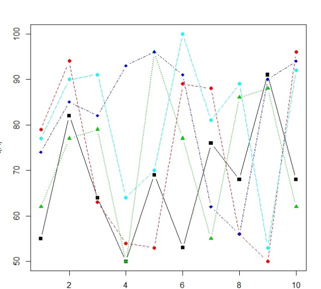
Imagine the following problem: You have a business assembling cabinets. You have 10 employees and you want to see who is the most efficient. You track the number of cabinets assembled by each employee over 10 days. You also track the hours they worked each day in a separate table.

Let’s create our tables –

Number of Cabinets

Create a vector of 100 random data points from 50 to 100.

# created random set of 100 numbers between 50 and 100
x <- sample(50:100,100, T)
x

sample(range,number of data, allow repeat of data (T,F))

matrixOps.jpg

Convert to a matrix

# convert to a 10x10 matrix
A <- matrix(x,10,10)
A

matrixOps1.jpg

Name Columns and Rows

#name rows and columns
colnames(A) <- c("D1","D2","D3","D4","D5","D6","D7","D8","D9","D10")
row.names(A) <- c("Bob","Steve","Gary","Sara","Tony","Stacey","Kerri","Debbie","George","Manny")
A

matrixOps2.jpg

Hours Worked

Let’s do the same thing, but now build our hours table.

# created random set of 100 numbers between 1 and 9
y <- sample(1:9,100, T)
y

matrixOps3.jpg


Convert to 10×10 matrix form

# convert to a 10x10 matrix
B <- matrix(y,10,10)
B

matrixOps4.jpg

Name our columns and rows

#name rows and columns
colnames(B) <- c("D1","D2","D3","D4","D5","D6","D7","D8","D9","D10")
row.names(B) <- c("Bob","Steve","Gary","Sara","Tony","Stacey","Kerri","Debbie","George","Manny")
B

matrixOps5.jpg

Matrix Operations

Now we will see the magic of R. This programming language was built for Statisticians. So it has some great matrix operations that make linear algebra operations a breeze. In fact, if you ever took linear algebra, you will wish you had known about R back then.

Now if I want to know how many cabinets each person made per hour worked on any given day, I would need to divide each elements of matrix A by its corresponding element in matrix B.

Taking what you know about For loops, think for a minute what the loop would look like to complete this task. Messy huh?

Well in R, we don’t have to worry it. Because in a R, A/B does just what we are asking for.

#matrix division
C = A/B
C

matrixOps6.jpg

The results are bit much, let’s round it to 1 decimal place

#round Matrix
round(C, digits =1)

matrixOps7.jpg

Okay, now let’s find the most and least productive values

#most and least
max(C)
min(C)

So we have one person who made 97 cabinets in an hour and another who made 6.875

matrixOps8.jpg

Who are they? And what day was it?

#who are they?
which(C==max(C), arr.ind=T)
which(C==min(C), arr.ind=T)

Manny is our hero on day 10, and Sara must have been hung over on day 10

matrixOps9

What about a mean?

I know, I know, if you are here, then you like me are a stat geek. So let’s run the mean and see who is the overall Rockstar.

#get the means
colMeans(C)
rowMeans(C)

I have underlined highest and lowest, both day and employee. Looks like Sara is a real slacker.

matrixOps10.jpg

Now before you start sending hate mail and calling me sexist, remember these numbers were randomly generated. If I ran my code again, I would get completely different answers. Just as if you follow along, your answers will not match up with mine.

The Code

# created random set of 100 numbers between 50 and 100
x <- sample(50:100,100, T)
x
# convert to a 10x10 matrix
A <- matrix(x,10,10)
A
#name rows and columns
colnames(A) <- c("D1","D2","D3","D4","D5","D6","D7","D8","D9","D10")
row.names(A) <- c("Bob","Steve","Gary","Sara","Tony","Stacey","Kerri","Debbie","George","Manny")
A

# created random set of 100 numbers between 1 and 9
y <- sample(1:9,100, T)
y
# convert to a 10x10 matrix
B <- matrix(y,10,10)
B
#name rows and columns
colnames(B) <- c("D1","D2","D3","D4","D5","D6","D7","D8","D9","D10")
row.names(B) <- c("Bob","Steve","Gary","Sara","Tony","Stacey","Kerri","Debbie","George","Manny")
B

#matrix division
C = A/B
C

#round Matrix
round(C, digits =1)

#most and least productive values
max(C)
min(C)

#who are they?
which(C==max(C), arr.ind=T)
which(C==min(C), arr.ind=T)

#get the means
colMeans(C)
rowMeans(C)


R: ANOVA (Analysis of Variance)

Performing an ANOVA is a standard statistical test to determine if there is a significant difference between multiple sets of data. In this lesson, we will be testing the readings of 4 sensors over the span of a year.

To play along, you can download the CSV file here: sensors

Load our library

library(HH)

Anova1

Let’s get the data into R

 mydata <- read.csv(file.choose())
 head(mydata)

Anova.jpg

Let’s make our data set a bit more user friendly by giving our sensors names (S1,S2,S3,S4)

row.names(mydata) <- c("S1","S2","S3","S4")
head(mydata)

Anova1.jpg

Now, our data is in cross tab format. Great for human reading, but not for machine. We need to adjust our data a little.

#transpose the data
mydataT <- t(mydata)
mydataT

Anova2

Now we need to stack the data. Before we can do that though, we need to convert it from a matrix to a dataframe

mydataDF <- as.data.frame(mydataT)

Now let’s stack() our data

myData1 <- stack(mydataDF)
head(myData1)

Anova3

stack() makes your data more computer readable. Your column names are turned into elements in a column called “ind”

Now let’s test our data

I know there were a lot of steps getting here, but I want to assure you that your data will never come in the format you need it in. You will always have to do some sort of manipulation to get it in the format you need.

Box plot (box-whisker plot)

Box plots are a great way to visualize multiple data sets to see how they compare.

bwplot(values ~ ind, data = myData1, pch="|")

Anova4.jpg

Take a look at S3, look at how offset it looks – The median doesn’t even cross the 1-3 quartiles of S1,S2, or S4

Anova5.jpg

But is this difference significant?

What do I mean by significant? Well, the easiest way for me to explain significance in this case is – can the difference shown above be repeated by random chance? If I took another sampling of the readings would this difference be present or would maybe a difference sensor be out of range?

We use a test called ANOVA (Analysis of Variance) to find out:

ANOVA (one way)

The code in this case is simple enough

myData1.fix.aov <- aov(values ~ ind, data=myData1)
anova(myData1.fix.aov)

It is the results I want to spend a moment on

Anova6

Df of ind= 3 – degrees of freedom – calculated by (4 Sensors – 1)

Df Residuals =44 – this is calculated by total row 48 – 4(the 4 sensors used above)

Sum Sq and Mean Sq = Sum of Squares and Mean Sum of Squares. I am not going to go into the math here, but these two values are calculated comparing the means between our 4 sensors.

You use the Sum Sq and Mean Sq to calculate the F value. You then go find an F chart like the one here: link

You will look up the F ratio (3,44) 3 across, 44 down. These numbers come from the Df( degrees of freedom column). If you look on the table, you will see an F value of 2.82. Our value is 7.4195 WAYYY more than 2.82. This means our ANOVA test proves significance.

It should be noted that the ANOVA test does not tell which sensor is the one out of range. In fact, you could have one or two sensors out of range. We do not know yet. All we know is that something is significantly different.

p-value

Now I know there are some Stat savvy people reading this who are just dying for me to point out the obvious.

Anova7.jpg

The value circled above is your p value. Most standard significance tests use 0.1 or 0.05 as a value to shoot for. If your p-value comes under these values, you have something. Our p-value is 0.0003984 – way under. We definitely found proof of variance.

mean-mean comparison

Now let’s see what values are different. To do this, we can use a mean-mean comparison chart.

model.tables(myData1.fix.aov, "means")
myData1.fix.mmc <- mmc(myData1.fix.aov, linfct = mcp(ind = "Tukey"))
myData1.fix.mmc
mmcplot(myData1.fix.mmc, style = "both")

You can review the Tukey values below

Anova8.jpg

But I prefer just looking at the chart. To get a quick understanding of how to read this chart, look at the vertical dotted line down the center of the chart. This is the zero line. Now look at the horizontal lines. All the black ones cross the zero line – they are within range of each other.

Look at the red lines now. These are our lines that include S3. It is the means comparisons with S3 that don’t cross the zero line.

This tells you that S3 is the sensor out of range

Anova9

Looking back at our box-whisker plot, this really isn’t a surprise

Anova5

HOV – Brown Forsyth

Finally to confirm our one-way Anova, we have one more test to pass. That is the the homogeneity of variance (Brown Forsyth) test.

In order for a F-test to be valid, the group variances within data must be equal.

hovBF(values ~ ind, data=myData1)
hovplotBF(values ~ ind, data=myData1)

Again, I am not going to go into the math, just show you how to read it.

the HOV plot runs difference measures of the spreads of the variances from each sensor from the group median. As you can see in the middle and right plots, the boxes all overlap each other. In a failed HOV, one of the medians in the right plot would not over lap the other 3 boxes.

Anova11.jpg

In an HOV, looking at our p-value is once again the quickest approach. The p-value here is 0.14 – well above normal significance levels of 0.10 and 0.05.

So, this means there is no reason to disclaim our F-test.

Anova10.jpg

So to wrap up everything above, you want a low P value for your F-test and a high P-value for your HOV.

Sorry if you head is spinning a little here. The goal of my site is to go light on the math and show you how to let the computer do the work.

The Code

library(HH)

#get data
mydata <- read.csv(file.choose())
head(mydata)

#name rows
row.names(mydata) <- c("S1","S2","S3","S4")
head(mydata)

#transpose data
mydataT <- t(mydata)

#change to dataframe
mydataDF <- as.data.frame(mydataT)

#stack your data
myData1 <- stack(mydataDF)
head(myData1)

#box whisker plot
bwplot(values ~ ind, data=myData1)

#anova
myData1.fix.aov <- aov(values ~ ind, data=myData1)
anova(myData1.fix.aov)

#mmc
model.tables(myData1.fix.aov, "means")
myData1.fix.mmc <- mmc(myData1.fix.aov, linfct = mcp(ind = "Tukey"))
myData1.fix.mmc
mmcplot(myData1.fix.mmc, style = "both")

# homogeneity of variance – Brown Forsyth
hovBF(values ~ ind, data=myData1)
hovplotBF(values ~ ind, data=myData1)


R: Boxplot – comparing data

We are going to make some box plots in R to compare readings of 4 sensors over 1 calendar year.

To play along, download the CSV file here: sensors

HH

First, call library(HH) – if HH won’t load, you may need to install the package: R: Installing Packages

Data

First, let us import the CSV file. Using the following command, R will open a window allow you to search for your file.

SenData  <- read.csv(file.choose())

boxplot.jpg

Using the head() command, let’s look at our data.

What we have is monthly readings for 4 sensors (1-4)

boxplot1.jpg.

Our data is in tabular (often called cross-tab) format This is great for human readability, but computers don’t really like it.

Let’s use stack() to change our data into a computer friendly format.

boxplot2.jpg

Boxplot

using bwplot – we are going to plot values against “ind” – months. Note we set out data to the SenD matrix

boxplot3

What we get is the box plot below

boxplot4.jpg

a box plot – or box and whisker plot – provides a graphical representation of the median as well as 1rst,2nd,3rd and 4th quartiles. Lining them up lets you see how data in each unit compare to each other.

boxplot6.jpg

Let’s add some color to the chart.

boxplot7.jpg

boxplot8.jpg

Notice the month are in alphabetical order. Let’s fix that.

boxplot9

boxplot10

Let’s break our time frame into quarters now.

To better understand the code

  • SenD$quarter <- creates a new variable named quarter
  • factor() — creates a factor
  • c() – creates a vector
  • rep(1,12) … – repeats 1 twelve times then 2 twelve times, etc.
  • We use 12 because we have 3 months in a quarter, and 4 sensors per month 3*4 = 12

boxplot12.jpg

boxplot11

Here is some code to plot our quarters. I think if you look at the code and plot, you should be able to make out most of the additions.

**hint pch=8 turns the median line into “*”

boxplot13

boxplot14.jpg