Python: Read CSV and Excel with Pandas

Earlier is showed you how to use the Python CSV library to read and write to CSV files. While CSV does work, and I still use elements of it occasionally, you will find working with Pandas to be so much easier.

Practice Files Excel: Linear Regression Example File 1

CSV: heightWeight_w_headers

Let’s start with our CSV file. Unzip it and place it in a folder where you will be able to find it.

If you want to make your life a little easier, when you open your Jupyter Notebook, type pwd

This will give you your present working directory. If you place your csv file in this directory, all you have to do is call it by name.

csv1

I am not going to do that however. I want to show you how to work with directories.

Get Full Directory Path

For Windows Users, if you hold down the Shift key while right clicking on your file, you will see an option that says: Copy as Path

csv2

Read the CSV file

First import pandas as pd

Then assign a variable = pd.read_csv(file name) – paste the full path of your CSV file here.

variable.head() = the first 5 rows from your data frame.

pandaCSV

Write CSV file

Okay, let’s write a CSV file. First, let’s add some rows to current dataframe.

We will do this be first creating a new dataframe with 3 rows of data.

pandaCSV1.jpg

Now we will use the .append() function to append this new dataframe to end of our existing dataframe.

The ignore_index = True argument tells the new rows to continue using the index of the main dataframe. Otherwise, the new rows would start counting at 0 again. If you want to try it, just leave out the argument: HgtWgt_df.append(df2)

pandaCSV2.jpg

Now, we just use the df.to_csv() command to write our appended dataframe to a new CSV file

pandaCSV3

And there is our new file

pandaCSV4.jpg

Read Excel File

I’d love to be able to wow you with how complicated reading an Excel file is, but the difference between the Excel file reading and CSV is one word – excel.

pandaexcel.jpg

The only caveat is if your Excel file has multiple sheets. By default pd.read_excel() goes to sheet 1. If you want it to read sheet 4 instead, you would add: pd.read_excel(filename, sheetname= 4)

Write to Excel File

pandaexcel1.jpg

Bonus note

If you haven’t already, please check out my earlier CSV lesson: Python: Working with CSV Files

This will really give you an appreciation for how powerful and time saving pandas really is.


If you enjoyed this lesson, click LIKE below, or even better, leave me a COMMENT. 

Follow this link for more Python content: Python


Python: Co-variance and Correlation

In this lesson, I will using data from a CSV file. You can download the file here: heightWeight

If you do not know how to import CSV files into Python, check out my lesson on it first: Python: Working with CSV Files

The Data

The data set includes 20 heights (inches) and weights(pounds). Given what you already know, you could tell me the average height and average weight. You could tell me medians, variances and standard deviations.

correl

But all of those measurements are only concerned with a single variable. What if I want to see how height interacts with weight? Does weight increase as height increases?

**Note while there are plenty of fat short people and overly skinny tall people, when you look at the population at large, taller people will tend to weigh more than shorter people. This generalization of information is very common as it gives you a big picture view and is not easily skewed by outliers.

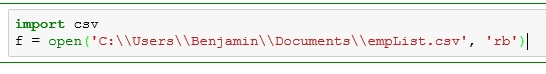
Populate Python with Data

The first thing we are going to focus on is co-variance. Let’s start by getting our data in Python.

correl1.jpg

Now there is a small problem. Our lists are filled with strings, not numbers. We can’t do calculations on strings.

We can fix this by populating converting the values using int(). Below I created 2 new lists (height and weight), created a for loop counting up to number of values in our lists : range(len(hgt)). Then I filled the new lists using lst.append(int(value))

correl2.jpg

**Now I know I could have resolved this in fewer steps, but this is a tutorial, so I want to provide more of a walk through.

Co-variance

Co-variance tells us how much two variables disperse from the mean together. There are multiple ways to find co-variance, but for me, using a dot product approach has always been the simplest.

For those unfamiliar with dot product. Imagine I had 2 lists (a,b) with 4 elements each. The dot product with calculated as so: a[0]*b[0]+a[1]*b[1]+a[2]*b[2]+a[3]*b[3]

Here is how it works:

If I take the individual variance of height[0] and weight[0] and they are both positive or negative – the product will be positive. – both variables are moving in the same direction

One positive and one negative will be negative. The variables are moving in different directions

One you add them all up, a positive number will mean that overall, you variables seem to have a positive co-variance (if a goes up, b goes up – if a goes down, b goes down)

If the final result is negative, you have negative co-variance (if a goes up, b goes down – if a goes down, b goes up)

If your final answer is 0 – your variables have no measurable interaction

Okay, let’s program this thing

** we will be using numpy’s mean() – mean and dot() – dot product methods and corrcoef() – correlation coefficient

First we need to find the individual variances from mean for each list

I create a function called ind_var that uses a list comprehension to subtract the mean from each element in the list.

correl3.jpg

Now, let’s change out the print statement for a return, because we are going to be using this function inside another function.

correl4.jpg

Co-variance function

Now let’s build the co-variance function. Here we are taking the dot product of the variances of each element of height and weight. We then divide the result by the N-1 (the number of elements – 1 : the minus 1 is due to the fact we are dealing with sample data not population)

correl6

So what were are doing:

  • Take the first height (68 inches) and subtract the mean (66.8) from it (1.2)
  • Take the first weight (165 lbs) and subtract the mean(165.8)  from it (-0.8)
  • We then multiply these values together (-0.96)
  • We repeat this for each element
  • Add the elements up.
  • Divide by 19 (20-1)
  • 144.75789 is our answer

Our result is 144.75789  – a positive co-variance. So when height goes up – weight goes up, when height goes down – weight goes down.

But what does 144 mean? Not much unfortunately. The co-variance doesn’t relate any information as to what units we are working with. 144 miles is a long way, 144 cm not so much.

Correlation

So we have another measurement known as correlation. A very basic correlation equation divides out the standard deviation of both height and weight. The result of a correlation is between 1 and -1. With -1 being perfect anti-correlation and 1 being perfect correlation. 0 mean no correlation exists.

With my equation get 1.028  – more than one. This equation is simplistic and prone to some error.

correl7.jpg

numpy’s corrcoef() is more accurate. It shows us a correlation matrix. Ignore the 1’s – they are part of what is known as the identity. Instead look at the other numbers = 0.97739.  That is about as close to one as you will ever get in reality. So even if my equation is off, it isn’t too far off.

correl9

Now just to humor me. Create another list to play with.

correl10

Let’s run this against height in my correlation function

correl11.jpg

Run these value through the more accurate corrcoef() . This will show my formula is still a bit off, but for the most part, it is not all that bad.

correl8


If you enjoyed this lesson, click LIKE below, or even better, leave me a COMMENT. 

Follow this link for more Python content: Python


Python: Working with CSV Files

Since you are on my site, I am going to go out on a limb here and say you are interested in working with Data in one form or another. I mean, if you are looking to learn how to make a video game with Python, you are in the wrong place. I am not going to be much help to you at all.

But, for those of us who do want to work with data, the last thing we want to do have to manually input all the data. We need methods for reading from and writing to files and databases. We will start by learning to read and write a CSV  (comma separated values) file.

If you would like to play along, you can download the CSV file I will be working with here: empList

Unzip the file and place it somewhere you can find it.

The file contains 7 records, with 3 columns each.

csv

If you want to make your life a little easier, when you open your Jupyter Notebook, type pwd

This will give you your present working directory. If you place your csv file in this directory, all you have to do is call it by name.

csv1

I am not going to do that however. I want to show you how to work with directories.

Get Full Directory Path

For Windows Users, if you hold down the Shift key while right clicking on your file, you will see an option that says: Copy as Path

csv2

CSV Module

To read or write to a CSV file, you need to import the CSV module.

In the next line I use the open() method from the CSV module to open my file.

f = open(paste your file path you copied here, ‘rb’)‘rb’ is required for reading CSV files in Python 2.7

Note the double \\ . I had to add the second \ to my copied file path. If you don’t Python will view the single \ as an escape character and your file will not open.

csv3.jpg

Read the file

Now that the file has been opened, let’s read it. We start by passing the file through the csv.reader() method

Now we can work with it. Below I use a for loop to iterate each row in the file.

csv4.jpg

You can pick and choose columns like you would reading from a list (using indexes).

Notice I had to import the file again – once CSV iterates through a file, you need to re-import it use it again.

csv5.jpg

You can dump the file into variables though. You can work on those variables repeatedly. In the example below I dump each column into a list.

csv56.jpg

Write a CSV file

Writing a csv file is pretty simple as well. However, when opening the file, use ‘wb’ as the second argument, not ‘rb’.

In this example, I am creating a new file ‘empList1.csv‘ and placing the values found in my Name list in the file.

writing in CSV requires you to use the csv.writer() command to make a writable object and use writerow() just like you did readrow()

also, make sure to close() the file or you will not be able to access it later.

csv57.jpg

There is a problem here though, look at the output. Python separated each letter in the names into their own columns.

csv58.jpg

The CSV file looks like this in Excel

csv59.jpg

Not exactly what I wanted.

The fix is square brackets [] inside the writerow().

csv60

Now our file is how we want it.

csv61


If you enjoyed this lesson, click LIKE below, or even better, leave me a COMMENT. 

Last Lesson: Python: Working with Rows in DataFrames

Next Lesson:

Return to: Python for Data Science Course

Follow this link for more Python content: Python


Python: Lists and Dictionaries

Lists and Dictionaries are kind of like super variables. They allow you to store multiple data under a singular name. In the example below, I first assign the variable ‘a‘ a value of 6. Next when I go to assign it a value of 7, it replaces 6.

What if I want to keep both 6 and 7?

pylist

Sure I could use 2 variables, (ex. a and b), or I can use a list.

List

A list is a collection of data in Python. You create a list by assigning a variable a group of data enclosed in square brackets [].

Notice that lists are indexed, meaning you call them up using the following syntax: variable[index]

Note that indexes in Python start at 0. So in our set of 4 elements, the indexes would be 0,1,2,3. Notice when I try to use index 4, I get an out of range error.

Screenshot 2022-07-04 210407

Lists can also hold strings, or combinations of values in one list.

Screenshot 2022-07-04 210637

Try your code in our online Python console:  

Adding and removing elements from a list

.append(): adds a element to the list

.pop(): removes last element from list

.remove(value): removes element matching value

del list[index]: deletes element by index

.clear(): removes all elements

Screenshot 2022-07-04 220540

Try your code in our online Python console:  

Dictionaries

This of dictionaries as lists with named indexes. This makes looking up values easier (especially when your code get more complicated).

Each data element is paired with a named index. A dictionary is denoted through the use of curly braces {} and : separating the named index and the value.

Screenshot 2022-07-04 210916


Try your code in our online Python console:  

If you enjoyed this lesson, click LIKE below, or even better, leave me a COMMENT. 

Last Page: Printing with .format{}

Next Page: Working with lists

Back to Python Course: Course

Python: Central Limit Theorem

The Central Limit Theorem is one of core principles of probability and statistics. So much so, that a good portion of inferential statistical testing is built around it. What the Central Limit Theorem states is that, given a data set – let’s say of 100 elements (See below) if I were to take a random sampling of 10 data points from this sample and take the average (arithmetic mean) of this sample and plot the result on a histogram, given enough samples my histogram would approach what is known as a normal bell curve.

In plain English

  • Take a random sample from your data
  • Take the average of your sample
  • Plot your sample on a histogram
  • Repeat 1000 times
  • You will have what looks like a normal distribution bell curve when you are done.

hist4

For those who don’t know what a normal distribution bell  curve looks like, here is an example. I created it using numpy’s normal method

hist5.jpg

If you don’t believe me, or want to see a more graphical demonstration – here is a link to a simulation that helps a lot of people to grasp this concept: link

Okay, I have bell curve, who cares?

The normal distribution of (Gaussian Distribution – named after the mathematician Carl Gauss) is an amazing statistical tool. This is the powerhouse behind inferential statistics.

The Central Limit Theorem tells me (under certain circumstances), no matter what my population distribution looks like, if I take enough means of sample sets, my sample distribution will approach a normal bell curve.

Once I have a normal bell curve, I now know something very powerful.

Known as the 68,95,99 rule, I know that 68% of my sample is going to be within one standard deviation of the mean. 95% will be within 2 standard deviations and 99.7% within 3.

hist.jpg

So let’s apply this to something tangible. Let’s say I took random sampling of heights for adult men in the United States. I may get something like this (warning, this data is completely made up – do not even cite this graph as anything but bad art work)

hist6.jpg

But reading this graph, I can see that 68% of men are between 65 and 70 inches tall. While less than 0.15% of men are shorter than 55 inches or taller than 80 inches.

Now, there are plenty of resources online if you want to dig deeper into the math. However, if you just want to take my word for it and move forward, this is what you need to take away from this lesson:

p value

As we move into statistical testing like Linear Regression, you will see that we are focus on a p value. And generally, we want to keep that p value under 0.5. The purple box below shows a p value of 0.5 – with 0.25 on either side of the curve. A finding with a p value that low basically states that there is only a 0.5% chance that the results of whatever test you are running are a result of random chance. In other words, your results are 99% repeatable and your test demonstrates statistical significance.

hist7.jpg

Python: Histograms and Frequency Distribution

In the spirit total transparency, this is a lesson is a stepping stone towards explaining the Central Limit Theorem. While I promise not to bog this website down with too much math, a basic understanding of this very important principle of probability is an absolute need.

Frequency Distribution

To understand the Central Limit Theorem, first you need to be familiar with the concept of Frequency Distribution.

Let’s look at this Python code below. Here I am importing the module random from numpy. I then use the function random_integers from random. Here is the syntax:

random.random_integers(Max value, number of elements) 

So random.random_integers(10, size =10) would produce a list of 10 numbers between 1 and 10.

Below I selected 20 numbers between 1 and 5

hist1.jpg

Now, since I am talking about a Frequency Distribution, I’d bet you could infer that I am concerned with Frequency. And you would be right. Looking at the data above, this is what I have found.

I create a table of the integers 1 – 5 and I then count the number of time (frequency) each number appears in my list above.

hist2.jpg

Histogram

Using my Frequency table above, I can easily make a bar graph commonly known as a histogram. However, since this is a Python lesson as well as a Probability lesson, let’s use matplotlab to build this.

The syntax should be pretty self explanatory if you have viewed my earlier Python graphing lessons.

hist3

Now lets, do it with even more data points (100 elements from 1 to 10 to be exact)

hist4.jpg


If you enjoyed this lesson, click LIKE below, or even better, leave me a COMMENT. 

Follow this link for more Python content: Python


Python: Arithmetic, Relational Operators, and Variables

Arithmetic Operators

Python Arithmetic Operators are pretty standard.

Arithmetic Operators

  • + : Addition
  • – : Subtraction
  • * : Multiplication
  • / : Division
  • //: Integer Division (Return divisor: 5/2 = 2)
  • % : Modulus (returns the remainder of a division problem: 5%2=1)
  • ** : Exponent (4**2 = 16)

Screenshot 2022-07-05 124159

Try your code in our online Python console: 

Relational Operators

Relational operators compare values and return a Boolean result (Boolean means 2 states, in this case True or False). Note when using relational operators, == is equal to. A single = is used to set a variable value, not to compare two values

> Greater than

< Less Than 

== Equal to

!= not equal

>= or <= greater than or equal, less than or equal

Screenshot 2022-07-05 122503

Try your code in our online Python console: 

Variables

Variables are a way of holding values in a program. You take a unique character string and you can assign values to it, and use the string throughout your program. Variables in Python are pretty straight forward. Unlike other programming languages, you do not need to define the variables first. Python dynamically assigns the data type.

Three main rules:

  • Variables must start with a letter or _
  • Variables are case sensitive
  • Avoid using command keywords (print, def, for)

pythonFundamentals3

notice lowercase ‘a‘ returns an error

Remember, Jupyter notebooks only return the last command. If you want both variables, use the print command

Screenshot 2022-07-03 210654

You can perform arithmetic functions on variables

Screenshot 2022-07-03 211010

And of course, variables can hold strings as well

Screenshot 2022-07-05 122935

Try your code in our online Python console: 

Last Lesson: Install Python and Hello World

Next Lesson: Print Variables and User Input

Back to Python Course: Course

8 Fun Facts About Python

  1. Python was named after the comedy troupe Monty Python. That is why you will often see spam and eggs used as variables in examples (a little tip of the hat to Monty Python’s Flying Circus)
  2. Python was created in 1991 by Guido Van Rossum
  3. There are Java and C variants of Python called JPython and CPython
  4. Python is an interpretive language, meaning you don’t need to compile it. This is great for making programs on the fly, but does make the code rather slow compared to compiled languages
  5. Python is part of the open source community, meaning plenty of independent programmers are out there building libraries and adding functionality to Python.
  6. It is one of the official languages at Google
  7. Ever work with Java or C? If so, one the first things you will notice is that Python has done away with braces. And it appears they even have a sense of humor about it. Look what happens when you try importing braces.pyfun
  8. Finally import this pyfun1.jpg

If you enjoyed this lesson, click LIKE below, or even better, leave me a COMMENT. 

Follow this link for more Python content: Python


Python: Fun with Central Tendency

Now numpy provides easy functions for finding central tendency – you can find them in my Numpy Part II lesson: Python: Numpy Part II.

But we have learned enough about Python so far, that maybe it would be more fun to build our own functions. In this lesson we are going to build our own statistics library with mean, median, mode, and quantile

Our Data

pythonCent

Mean

pythonCent1.jpg

or even easier:

pythonCent3

Median

Remember with median – if your data contains an odd number of elements (n%2==1), you just take the middle value. However, if your data contains and even number of elements (n%2==0) then you add the two middle numbers and divide by 2.

We handle that through the use of an if statement in our function.

pythonCent2

Mode

For mode, we want to find the most common element in the list. For this task, I will import Counter from collections.

d.most_common() returns each unique element and the number of times it appears

d.most_common(1) returns the

pythonCent4.jpg

or in function form:

pythonCent5.jpg

In my numpy part II lesson I use a more elegant solution, but I want you to see that there is always more than one way to do something in Python.

Quantile

Quantiles are cut points in set of data. They can represent the bottom ten percent of the data or the top 75% or any % from 0 to 100.

In my solution, I am adding a slicing argument to the sorted() function. Below shows all elements up to (but not including) index 4

pythonCent6

quantile function:

pythonCent7


If you enjoyed this lesson, click LIKE below, or even better, leave me a COMMENT. 

Follow this link for more Python content: Python

Python: Pandas, Working with DataFrames

Sure DataFrames look nice, but how can I work with them?

Let’s cover some basic tasks in pandas to get you started.

Let’s start by building a DataFrame

pyDF1

I don’t like where they placed Age on my dataframe. I want to move it.

To do so, we are going to cover a couple of new terms: axis, drop() and insert()

Axis

Using numpy and pandas, you will come across many functions that require you to enter an axis as a parameter. Axis 0 is your rows while Axis 1 is your columns. This is due to the way matrices are named with a 3×2 matrix having 3 rows and 2 columns and a 2×3 having 2 rows and 3 columns

pyDF2

drop()

To move the age column, I am first going to create a copy of my dataframe minus the age column. To do this, I am going to use the drop() function. The drop() function accepts two arguments drop(name, axis). In our case name = ‘Age’ and axis = 1 since we are referring to a column.

pyDF3

insert()

Now we want to insert the age column. The syntax for the insert() function is insert(insert point, name, data)

pyDF4

add a new column

Adding a new column is straight forward. Just DataFrame[new column name] = value.

Below I created at new column called ‘Age When Start’ that shows the age of employees when they started. I derived this value by subtracting Years Service column from Age column.

pyDF5.jpg

boolean column

You can create a boolean column using a boolean operator.

pyDF6

sort()

You can sort a dataframe by any column using sort_values()

pyDF7.jpg

Sort is set to ascending by default. To reverse it, set ascending = False

** remember in Python, True and False need to start with a capital letter.

pyDF8.jpg

slicing

by rows

slicing by rows is just like with a list

pyDF9

by columns

slicing by columns is a bit more complex. To slice by column name you have to use the dataframe.ix command.

pyDF10


If you enjoyed this lesson, click LIKE below, or even better, leave me a COMMENT. 

Last Lesson: Pandas DataFrames

Next Lesson: Pandas: Rename a Column

Return to: Python for Data Science Course

Follow this link for more Python content: Python