Data Jobs: What does a Data Analyst Do?

Data Analysts get a bad wrap. With the advent of the Data Scientist, Data Analysts are often viewed as Data Scientists lite, however I feel that is not the honest case. Truth is, there is a lot of overlap between the two fields. I will dive deeper into what a Data Scientist is in a future article, but just know my opinion is the definition of Data Scientist as a job is still a bit fuzzy and I think the job title may eventually be broken into a few different titles to better define the differences.

Data Analyst

So what does a Data Analyst do?

A lot actually. You could put 10 data analysts into a room and you would get ten different answers to this question. So the best I can do here is make sweeping generalities. As the old saying goes “Your results may vary”

In general, data analysts perform statistical analysis, create reporting, run ad-hoc queries from data warehouses, create data visualizations, create and maintain dashboards, perform data mining, and create machine learning models (yes, ML is not only for data scientists). Their assignments are business driven. A data analysts is either embedded with a business unit (financial planning, fraud, risk management, cyber security, etc.) or working in a centralized reporting/analytics team. They use their skills to provide reporting and analytics for the business.

Tools used by Data Analysts

  • SQL – MySql, SQL Server, Oracle, Teradata, Postgres – whether simply querying a data warehouse or creating and managing a local data mart, data analysts need to be advanced SQL programmers
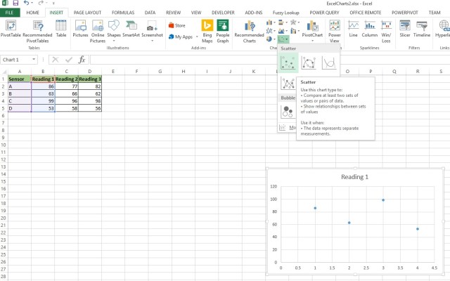
  • Visualization tools – Tableau, Qlik, Power BI, Excel, analysts use these tools to create visualizations and dashboards
  • Python/R – Data analysts should be familiar with languages like Python or R to help manage data and perform statistical analysis or build machine learning models
  • Spreadsheets – Excel, Google Sheets, Smart Sheets are used to create reports, and pivot tables used to analyze the data
  • ETL tools – SSIS, Alteryx, Talend, Knime, these tools are design to move data to and from databases, CSV files, and spreadsheets. Until the data is in a usable format, analysis cannot be performed.

Educational Requirements

Typically a data analyst position will ask for a bachelors degrees, preferably in computer science, statistics, database management or even business. While the barrier to entry for a data analyst job is generally not as high as a data scientist, that does not mean you cannot make a meaningful and well paid career as a data analyst. Also, the demand for data professionals seems to keep going up and up and it most likely will for the foreseeable future.

R: Importing Excel Files

To work with Excel files in R, you can use the readxl library

install.packages(“readxl”)

Use the read_excel() function to read and Excel workbook

> library(readxl)
>
> ## read excel file
> df1 <- read_excel("r_excel.xlsx")
> head(df1)
# A tibble: 6 x 4
  Name   Job              Hours Complete
  <chr>  <chr>            <dbl> <chr>  
1 Sally  Predictive Model    1. n      
2 Philip Maintanence        10. n      
3 Tom    Ad-hoc Report      12. y      
4 Bob    SSRS                3. y      
5 Philip Tableau             7. n      
6 Tom    Tableau             9. n

By default, read_excel() reads only the first sheet in the Excel file. To read other sheets using the sheet key word.

> ## read  sheet 2
> df2 <- read_excel("r_excel.xlsx", sheet =2)
> head(df2)

# A tibble: 6 x 2
  Animal Num_Legs
  <chr>     <dbl>
1 Dog          4.
2 Duck         2.
3 Snake        0.
4 Horse        4.
5 Spider       8.
6 Human        2.

The next example, we are reading range B2 – C6 on sheet 1 (same as Excel’s range function)

> ## read sheet 1, range B2 - C6
> df3 <- read_excel("r_excel.xlsx", sheet =1, range = "B2:C6")
> df3
# A tibble: 4 x 2
  `Predictive Model`   `1`
  <chr>              <dbl>
1 Maintanence          10.
2 Ad-hoc Report        12.
3 SSRS                  3.
4 Tableau               7.

In this last example, we are importing only the first 4 rows on sheet 2

> ## read sheet 2, first 4 rows only
> df4 <- read_excel("r_excel.xlsx", sheet = 2, n_max = 4)
> df4
# A tibble: 4 x 2
  Animal Num_Legs
  <chr>     <dbl>
1 Dog          4.
2 Duck         2.
3 Snake        0.
4 Horse        4.

Excel: Adjusting Named Ranges

Okay, so you created a spreadsheet. To make it easier for your fellow coworkers to use, you implemented range names. And it all works great, that is until you need to change the actual range.

Look at this example. I had created range call Class which spanned across 16 cells representing 16 classes being offered. It worked great until my boss informs me that my school will now be offering 20 classes.

You can download the Excel file here: ClassChoice

rangeAdj4.jpg

How do you change the range to include classes 17-20?

In the Formulas tab of the Ribbon, you will find an icon called Name Manager 

rangeAdj.jpg

Highlight the named range you are working with  – (in our case – Class)

Double click

rangeAdj1.jpg

Click on the little box to the right of the Refers to: box

rangeAdj2.jpg

Now highlight the new range

rangeAdj3

Click OK and OK. Now your range should contain your new cells.

Excel: Sorting and Filtering

Download Exercise File Here: ExcelTable

Sorting and Filtering are two basic functions you will perform quite often in Excel. When dealing with large data sets, it can be difficult to see what you are looking for, especially if the records appear in random order. Using sort and filter, you can adjust the spreadsheet to show what you want to see.

Sort

Sorting is simple in Excel. Just click on the header cell for the column you want to sort (in my example I chose “Name”). From the Ribbon Bar select Data. Now click on the AZ and ZA arrows. The column you selected will sort.

excelsort

Now, try it out on the other columns as well.

Finally, select the box directly above the word sort in the picture above. This will give you an advanced sort menu.

From this menu,  can select the column you wish to sort, the values you want to sort on, and the sort order.

excelsort1.jpg

Filter

To filter, select the Filter icon from the Data tab in the Ribbon Bar

excelsort2

Notice arrows now appear in the column header cells

excelsort3

Click on the arrow for Quarter. Now, uncheck the Select All box and check Quarter 2 > Okay

excelsort4.jpg

Now your sheet only has rows containing Quarter 2. Take note of the row numbers though. Notice the row numbers skip around. This is because the other rows are still there, they are just hidden by the filter.

excelsort5.jpg

Excel: An Introduction

Excel is Microsoft’s spreadsheet program. It is so well known, that for many the words Excel and spreadsheet are used interchangeably.

What is a spreadsheet? A spreadsheet is a computer program that uses columns and rows to store and perform calculations on data.

Notice in Excel, columns are denoted by letters and rows are denoted by numbers. The spaces are called cells. We refer to the cells by their letter and number designation. A1, B1,C2, etc.

excelIntro

Getting started, just click on A1 and enter “a”. Next click on B1 and enter 1.

Note how “a” hugs the left side of the cell and “1” hugs the right. This is because Excel automatically tries to define the data type in the cell. This this case, “a” is text and 1 is numeric.

excelIntro1

Now right click on the cell holding 1 (B1) and select Format Cells…

excelIntro2

From the pop up window, select Text and click okay. This converts 1 from Number to Text

excelIntro3

Now see how both cells hug the left.

excelIntro4

Cool Tricks

Excel has some cool tricks. I know most intro lessons don’t jump into what I am about to cover, but learning something cool always makes the learning process more fun.

Go to cell A3 and type “Monday”

Now notice the small green box in the bottom right corner of your cell. Click on that box, holding your mouse button key, drag your cursor down to A9

excelIntro5

How cool was that?

excelIntro6

Try it with month names.

excelIntro7

Now, trying it a number is a little different. Try placing 1 in a cell and dragging it down a couple cells. The numbers just repeat themselves.

excelIntro8

To get the numbers to work, type 1,2,3 in 3 consecutive cells.

excelIntro9

Highlight all 3 cells and click on the small green box. Now drag down a few cells and see what happens.

excelIntro10

Excel: Tables

Excel’s Table feature adds some nice functionality to your Excel workbook.

Download exercise file here: ExcelTable

Create Table

To create a table, highlight the cells you want and hit Ctrl-T. Leave My table has headers checked as our first row is header values.

exTab1.jpg

Your table will now look like this:

exTab2.jpg

The drop down menu in each header provides sorting and filtering.

exTab3

Tables provide a new set of menu items in the Ribbon Bar

exTab4

Let’s click the Total Row check box in the Ribbon Bar

exTab5

A Total Row will appear at the bottom of your table. You can select which kind of aggregate you want to perform.

exTab6

Slicer

Let’s add a slicer now.

exTab7.jpg

Select Name

exTab8.jpg

Now you have a slicer for your table.

exTab9

Now, select Charles and see how it filters your table

exTab10

Excel: Scatter Plots

Download worksheet here: ExcelCharts2

Our data set contains 3 sets of readings for 4 sensors (A,B,C,D)

excelCharts1

Scatter Plot

Reading 1

Highlight Columns A and B – From Ribbon > Insert>Scatter

excelCharts2.jpg

Here is a close up of the Scatter Plot icon

excelCharts3.jpg

Here is our plotting of Reading 1

excelCharts4

Reading 2

To add the Reading 2 column to the plot, right click on the chart area and Select Data

excelCharts5

Select Add

excelCharts6

  • Select the Heading from Column C for Series Name
  • A2:A5 as Series X values
  • C2:C5 as Series Y values

excelCharts7.jpg

Reading 3

Repeat again for Reading 3

excelCharts8

Now, double click on the Y-Axis and go to the Format Axis box that will appear on your right.

Select the Bar Chart Icon, and change the Axis Bounds to minimum of 40 and max of 100.

excelCharts9.jpg

This will help make the spacing between dots more pronounced. Generally altering a Y Axis away from 0 is considered bad taste as it tends to over-pronounce differences between elements.

excelCharts10

Now click on X-Axis and make the changes below.

excelCharts11

Next, go to Add Chart Element in the upper right corner. Legend>Right

excelCharts12

Here is our scatter plot

excelCharts13

Now wait a minute. I know what you are thinking, why is my X Axis 1 – 4 and not A,B,C,D

This is a flaw in Excel. There are some third party packages you can install that will allow you to rename the X Axis in a XY Scatter plot, but not with Excel in its default state.

You can however change the chart type to a Line Chart.

Go to Ribbon > Change Chart Type

Select Line

excelCharts14

Now your X-Axis is properly labeled

excelCharts15.jpg


Excel: Intro to Charts

Excel makes building basic charts easy.

Download sample data set here: ExcelCharts1

The Data

Our sample data set here is simple enough. We have 5 sensors (A,B,C,D,E) and one reading from each sensor.

excelChart

Column Chart

Let’s start with a column chart. To create a column chart, first select (highlight) your data set and then go to Insert>Column Chart in the Ribbon Bar.

excelChart1

From the column chart options, I am going to pick the first 2D chart option

excelChart2

excelChart3

Once a chart is created, you will notice a new element – Chart Tools – in the Ribbon Bar.

The first thing I want you to explore is Chart Styles. Click on the different options and see what happens.

excelChart4

Next, let’s try changing the colors:

excelChart5.jpg

Now go to Add Chart Element

Go to Axis Titles>Primary Horizontal

excelChart6

Now click on the Axis Title and rename it.

excelChart7

Label this Axis “Sensors”

excelChart8

Now select Primary Vertical and name it “Readings”

excelChart9

Now to change the chart title. Click on the title:

excelChart10

Rename it “Sensor Readings”

excelChart11


If you enjoyed this lesson, click LIKE below, or even better, leave me a COMMENT. 

Follow this link for more Excel content: Excel

Excel: Intro to Pivot Tables

Pivot Tables are a built in feature to Excel that allows for better data analysis. Using Pivot Tables, you can work with aggregates with ease.

Download this Excel file to follow along: studGrades

Let’s look at the data:

This data set represents Grades for 5 students across four quarters.

pivot1

Trying to calculate overall averages for each student or each class would require a lot of work using just straight spreadsheet functions. Pivot Tables make such tasks a breeze though.

Create a Pivot Table

Highlight you data set and go up to the Ribbon Bar > Insert>Pivot Table

pivot2

We are just going to hit OK here. But if you want to know a bit more about the window:

  • Choose the data that you want to analyze: notice the table range is A1 through F20 on the Courses tab. This is our data set.  – Use an external data source lets you grab your data from another program if you want
  • Choose where you want the PivotTable report to be place. – Default New Worksheet opens the table in a new sheet (our option) – Existing Worksheet allows you to place the table on an existing page
  • Choose whether you want to analyze multiple tables – this is more advanced. This lets you take multiple tables and join them together for analysis.

pivot3

After you click okay, Excel opens up your new Pivot Table

pivot4

Average Student Grade for Q1

Drag Stud_ID down to the ROWS box and Q1 down to Values

pivot5

Now we don’t want a Sum, we want an Average. So click on the down arrow by Sum of Q1 in VALUES. Select Value Field Settings…

pivot6

Now select Average and click OK

pivot7

Now you have averages in your table

pivot8

Average grades in classes

To find averages for classes, drag Stud_ID out of ROWS and drag Class into ROWS

pivot9

Now you have average grades for classes.

pivot10

The other 3 quarters

Just drag Q2, Q3, and Q4 into VALUES. Note they will most likely default as SUM, so you will need to change them to Average same way you did above.

pivot11

pivot12


If you enjoyed this lesson, click LIKE below, or even better, leave me a COMMENT. 

Follow this link for more Excel content: Excel

Excel: Data Cleaning

Data cleaning is one of the least enjoyable tasks for data professionals. Unfortunately, most data scientists I have spoken to state that data cleaning makes of 60% to 70% of their work load.

While there is no magic data cleaning machine I am aware of, there are some tips and tricks that you can learn to save you a lot of time and head aches. I have put together a 2 part video series using Excel that shows some of the most common data cleaning tasks:

  • Handling Duplicates
  • Spelling Errors
  • Missing Data
  • Converting Data
  • Merging Data Sets

I even have the Excel worksheet available for download so you can work along with the videos.

Download the file here: Data Cleaning

Videos

Below, you will find the links to my videos (video opens in new tab)

Excel: Data Cleaning with Excel Part 1 

Excel: Data Cleaning with Excel Part 2


If you enjoyed this lesson, click LIKE below, or better yet, leave me a COMMENT. 

Follow this link for more Excel content: Excel