Here is the data set if you want to play along: ExcelCharts2

While Excel does a pretty good job of auto-formatting charts based on your data, sometimes a little customization work is in order. Take this data below for example:

What if I want to create a bar chart of the average readings?

Well first we need to make an “Average” column

I really don’t need all the decimal places. Hit the decimal reduce button in the picture below until you have a column full of integers.

Chart Method 1

Just like you would normally, select all the data and go to Insert > Column Chart

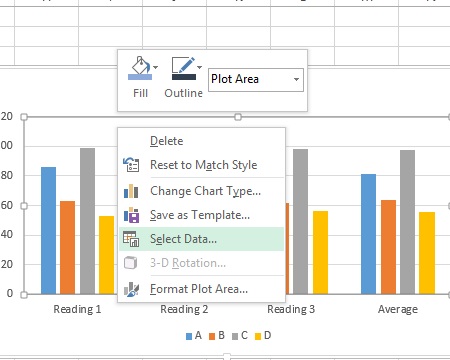
Right Click on your new chart and Select Data…

I don’t want my readings on the X axis, I want my Sensor Names, so click Switch Row/Column in the new window.

The X Axis is now A,B,C,D

Now, we only want to see the Average  column, so uncheck Reading 1,2,3 

Here is our chart

Chart Method 2

Don’t select any data yet. Just go to the Insert and Select Column Chart

Click Select Data now from the Ribbon (if you don’t see this, click anywhere on your new blank chart and this should appear in the Ribbon)

Click Add in the low left box.

In Series Name, either type a name or select the column header

In Series values: put put your data rows from the Average  column

Now we have data loaded into our chart, let’s change the data labels for our X Axis. In the Horizontal(Category) Axis Labels –  click Edit

Highlight A,B,C,D from the Sensor column

Now you see the numbers have been replaced by A,B,C,D

Here is our chart