R: K-Means Clustering- Deciding how many clusters

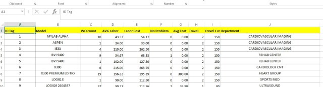
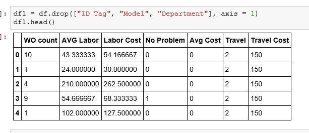
In a previous lesson I showed you how to do a K-means cluster in R. You can visit that lesson here: R: K-Means Clustering.

Now in that lesson I choose 3 clusters. I did that because I was the one who made up the data, so I knew 3 clusters would work well. In the real world it doesn’t work that way. Choosing the right number of clusters is one of the trickier parts of performing a k-means cluster.

If you go over to Michael Grogan’s site, you will see he has a great method for figuring out how many clusters to choose. http://www.michaeljgrogan.com/k-means-clustering-example-stock-returns-dividends/

wss <- (nrow(sample_stocks)-1)*sum(apply(sample_stocks,2,var))
for (i in 2:20) wss[i] <- sum(kmeans(sample_stocks,
centers=i)$withinss)
plot(1:20, wss, type="b", xlab="Number of Clusters",
ylab="Within groups sum of squares")

If you understand the code above, then great. That is a great solution for choosing the number of clusters. If, however, you are not 100% sure what is going on above, keep reading. I’ll walk you through it.

K-Means Clustering

We need to start by getting a better understanding of what k-means clustering means. Consider this simplified explanation of clustering.

The way is works is each of the rows our data are placed into a vector.

2016-12-06_22-09-28

These vectors are then plotted out in space. Centroids (the yellow stars in the picture below) are chosen at random. The plotted vectors are then placed into clusters based on which centroid they are closest to.

kmeans

So how do you measure how good your clusters fit. (Do you need more clusters? Less clusters)? One popular metrics is the Within cluster sum of squares. R provides this as kmeans$withinss. What this means is the distance the vectors in each cluster are from their respected centroid.

The goal is to get the is to get this number as small as possible. One approach to handling this is to run your kmeans clustering multiple times, raising the number of the clusters each time. Then you compare the withinss each time, stopping when the rate of improvement drops off. The goal is to find a low withinss while still keeping the number of clusters low.

2016-12-10_22-02-49

This is, in effect, what Michael Grogan has done above.

Break down the code

Okay, now lets break down Mr. Grogan’s code and see what he is doing.

wss <- (nrow(sample_stocks)-1)*sum(apply(sample_stocks,2,var))
for (i in 2:20) wss[i] <- sum(kmeans(sample_stocks,
centers=i)$withinss)
plot(1:20, wss, type="b", xlab="Number of Clusters",
ylab="Within groups sum of squares")


The first line of code is a little tricky. Let’s break it down.

wss <- (nrow(sample_stocks)-1)*sum(apply(sample_stocks,2,var))

sample_stocks – the data set

wss <-  – This simply assigns a value to a variable called wss

(nrow(sample_stocks)-1)  – the number of rows (nrow) in sample_stocks – 1. So if there are 100 rows in the data set, then this will return 99

sum(apply(sample_stocks,2,var)) – let’s break this down deeper and focus on the apply() function. apply() is kind of like a list comprehension in Python. Here is how the syntax works.

apply(data, (1=rows, 2=columns), function you are passing the data through)

So, let’s create a small array and play with this function. It makes more sense when you see it in action.

 tt <- array(1:20, dim=c(10,2)) # create array with data 1 -20, 
                                #10 rows, 2 columns
> tt
 [,1] [,2]
 [1,] 1 11
 [2,] 2 12
 [3,] 3 13
 [4,] 4 14
 [5,] 5 15
 [6,] 6 16
 [7,] 7 17
 [8,] 8 18
 [9,] 9 19
[10,] 10 20

Now lets try running this through apply.

> apply(tt, 2, mean)
[1] 5.5 15.5

Apply took the mean of each column. Had I used 1 as the second argument, it would have taken the mean of each row.

> apply(tt, 1, mean)
 [1] 6 7 8 9 10 11 12 13 14 15

Also, keep in mine, you can create your own functions to be used in apply

apply(tt,2, function(x) x+5)
 [,1] [,2]
 [1,] 6 16
 [2,] 7 17
 [3,] 8 18
 [4,] 9 19
 [5,] 10 20
 [6,] 11 21
 [7,] 12 22
 [8,] 13 23
 [9,] 14 24
[10,] 15 25

So, what is Mr. Grogan’s doing with his apply function? apply(sample_stocks,2,var) – He is taking the variance of each column his data set.

 apply(tt,2,var)
[1] 9.166667 9.166667

And by summing it: sum(apply(sample_stocks,2,var)) – he is simply adding the two values together.

 sum(apply(tt,2,var))
[1] 18.33333

So, the entire first line of code using our data is:

wss <- (nrow(tt)-1)*sum(apply(tt,2,var))

wss <- (10-1) * (18.333)

wss <- (nrow(tt)-1)*sum(apply(tt,2,var))
> wss
[1] 165

What this number is effectively is the within sum of squares for a data set that has only one cluster

Next section of code

Next we will tackle the next two lines of code.

for (i in 2:20) wss[i] <- sum(kmeans(sample_stocks,
centers=i)$withinss)

The first part is a for loop and should be simple enough. Note he doesn’t use {} to denote the inside of his loop. You can do this when your for loop is a single line, but I am going to use the {}’s anyway, as I think it makes the code a bit neater.

for (i in 2:20)  — a for loop iterating from 2 -20

for (i in 2:20) {

wss[i] <- }  – we are going to assign more values to the vector wss starting at 2 and working our way down to 20.

Remember, a single value variable in R is actually a single value vector.

c <- 5
> c
[1] 5
> c[2] <- 7
> c
[1] 5 7

Okay, so now to the trickier code. sum(kmeans(sample_stocks, centers = i)$withinss)

What he is doing is running a kmeans cluster for the data one time each for each value of centers (number of centroids we want) from 2 to 20 and reading the $withinss from each run. Finally it sums all the withinss up (you will have 1 withinss for every cluster you create – number of centers)

Plot the results

The last part of the code is plotting the results

plot(1:20, wss, type="b", xlab="Number of Clusters",
ylab="Within groups sum of squares")

plot (x, y, type= type of graph, xlab = label for x axis, ylab= label for y axis

Let’s try it with our data

If you already did my Kmeans lesson, you should already have the file, if not you can download it hear. cluster

 myData <- read.csv('cluster.csv')
> head(myData)
 StudentId TestA TestB
1 2355645.1 134 24
2 8718152.6 155 32
3 8303333.6 130 25
4 6352972.5 185 86
5 3381543.2 153 95
6 817332.4 153 81
> myData <- myData [,2:3] # get rid of StudentId column
> head(myData)
 TestA TestB
1 134 24
2 155 32
3 130 25
4 185 86
5 153 95
6 153 81

Now lets feed this through Mr. Grogan’s code

wss <- (nrow(myData)-1)*sum(apply(myData,2,var))
for (i in 2:20) {
          wss[i] <- sum(kmeans(myData,
          centers=i)$withinss)
         }
plot(1:20, wss, type="b", xlab="Number of Clusters",
ylab="Within groups sum of squares")

Here is our output ( a scree plot for you math junkies out there)

2016-12-11_14-05-39.jpg

Now Mr. Grogan’s plot a nice dramatic drop off, which is unfortunately not how most real world data I have seen works. I am going to chose 5 as my cut off point, because while the withinss does continue to decrease, it doesn’t seem to do so at a rate great enough to accept the added complexity of more clusters.

If you want to see how 5 clusters looks next to the three I had originally created, you can run the following code.

myCluster <- kmeans(myData,5, nstart = 20)
myData$cluster <- as.factor(myCluster$cluster)
ggplot(myData, aes(TestA, TestB, color = cluster))
+ geom_point()

5 Clusters

2016-12-11_14-13-02

3 Clusters

graph

I see some improvement in the 5 cluster model. So Michael Grogan’s trick for finding the number of clusters works.


R: K-Means Clustering

Note: This is an introductory lesson with a made up data set. After you are finished with this tutorial, if you want to see a nice real world example, head on over to Michael Grogan’s website:

http://www.michaeljgrogan.com/k-means-clustering-example-stock-returns-dividends/

K Means Cluster will be our introduction to Unsupervised Machine Learning. What is Unsupervised Machine Learning exactly? Well, the simplest explanation I can offer is that unlike supervised where our data set contains a result, unsupervised does not.

Think of a simple regression where I have the square footage and selling prices (result) of 100 houses. Taking that data, I can easily create a prediction model that will predict the selling price of a house based off of square footage. – This is supervised machine learning

Now, take a data set containing 100 houses with the following data: square footage, house style, garage/no garage, but no selling price. We can’t create a prediction model since we have no knowledge of prices, but we can group the houses together based on commonalities. These groupings (clusters) can be used to gain knowledge of your data set.

I think seeing it in action will help.

Here is the data set: cluster

The data we will be looking at test results for 149 students.

2016-12-06_22-09-28.jpg

The task at hand is to group the students into 3 groups based on the test results. Now one thing any teacher will let you know is that some kids perform well in one subject and perhaps not so well in another. So we can’t simply group them on the score performance on one test. And when you are dealing with real world data, you might be looking at 20 -100 test/quiz scores per student.

So what we are going to do is let the computer decide how to group (or cluster) them.

To do so, we are going to be using K-means clustering. K-means clustering works by choosing random points (centroids). It then groups the data points around the centroids based which centroid the points are closest to.

Let’s get started

Let’s start by loading the data

st <- read.csv(file.choose())
head(st)

our data

2016-12-06_22-23-40.jpg

Now let’s run the data through a Kmeans() algorithm

First, we are only going to want to focus on columns 2 and 3 in the data set since column 1 (studentID) is basically a label and provides no value in prediction.

To do this, we subset the data: st[,2:3] – which means I want all row ([,) and columns 2-3 (2:3])

2016-12-06_22-27-11.jpg

Now the code to make our clusters

stCl <- kmeans(st[, 2:3], 3, nstart = 20)
stCl

The syntax is kmeans(DATA, Number of clusters, Numbers of random starts)

Number of clusters I picked as 3 because I know this works well with the data, picking the right number usually takes a little trial and error in real life

Number of random starts is how many times you want the algorithm to be rerun (choosing new centroids each time) and choosing the result where the clusters are tightest.

Below is the output of our Kmeans – note the cluster means, this tells us the mean score for TestA and TestB set in each cluster.

2016-12-06_22-36-33.jpg

Hey, if you are a math junkie, this may be all you want. But if you are looking for some more practical value here, lets move on.

First, we need to add a column to our data set that shows our columns.

Now since we read our data from a csv, it is a data frame. If you can’t remember that, you can always run the command is.data.frame(st) to test it out.

Do you remember how to add a column to a data frame?

Well, there are multiple ways, but this is, in my opinion, the easiest way.

st$cluster <- stCl$cluster

is.data.frame(st)
st$cluster <- stCl$cluster
head(st)

Here is the result

2016-12-06_22-43-22.jpg

Now with the clusters, you can group your students based their assigned cluster.

Technically we are done here. We have successfully grouped the students. But what if you want to make sure you did a good job. One quick check is to graph your work.

Before we can graph, we have to make sure our st$cluster column is set as a factor, then using ggplot, we can graph it. (if you don’t have ggplot2 installed, you will need to run this line: install.packages(“ggplot2”)

library(ggplot2)
st$cluster <- as.factor(st$cluster)
ggplot(st, aes(TestA, TestB, color = cluster)) + geom_point()

And here is our output. The groups look pretty good.

graph.jpeg

Python: K Means Cluster

K Means Cluster will be our introduction to Unsupervised Machine Learning. What is Unsupervised Machine Learning exactly? Well, the simplest explanation I can offer is that unlike supervised where our data set contains a result, unsupervised does not.

Think of a simple regression where I have the square footage and selling prices (result) of 100 houses. Taking that data, I can easily create a prediction model that will predict the selling price of a house based off of square footage. – This is supervised machine learning

Now, take a data set containing 100 houses with the following data: square footage, house style, garage/no garage, but no selling price. We can’t create a prediction model since we have no knowledge of prices, but we can group the houses together based on commonalities. These groupings (clusters) can be used to gain knowledge of your data set.

I think seeing it in action will help.

If you want to play along, download the data set here: KMeans1

The data set contains a 1 year repair history of 197 Ultrasound medical devices.

Data dictionary (ID Tag – asset number assigned device, Model – model name of device, WO Count – count of repair work orders, AVG Labor – average labor minutes per repair, Labor Cost – average labor cost per repair, No Problem-  count of repairs where no problem was found, Avg Cost -average cost of parts, Travel – average travel hours per repair, Travel Cost – average travel cost per repair, Department – department that owns the ultrasound device)

kmeans

We want to see what kind of information we can extract from this data.

To do so, we are going to use K Means Clustering.

How does K Means Clustering work? Each row in the table is converted to a vector. Imagine the vectors now graphed in N-dimension space. Next pick the number of clusters you want to create. For each cluster, you will place a  point(a centroid) in space and the vectors are grouped based on their proximity to their nearest centroid.

The calculation to tell proximity is made using geometric means (not arithmetic)- hence the name K-Means Cluster

(each dot below is a row in your table, the colors represent a cluster)

kmeans2

Let’s do it in Python

Import the data.

import pandas as pd

df = pd.read_excel("C:\Users\Benjamin\Documents\KMeans1.xlsx")
df.head()

kmeans1

Now, we are going to drop a few columns: ID Tag – is a random number, has no value in clustering. Then Model and Department,as they are text and while there are ways to work with the text, it is more complicated so for now, we are just going to drop the columns

df1 = df.drop(["ID Tag", "Model", "Department"], axis = 1)
df1.head()

kmeans2

Now lets import KMeans from sklearn.cluster

We then initialize KMeans (n_clusters= 4 -no of clusters you want, init=’k-means++’ -sets how the centroids are places. k-means++ is one of the faster methods of centroid placement, n_init=10 – number times the algorithm with run placing new centroids each iteration)

from sklearn.cluster import KMeans
km = KMeans(n_clusters=4, init='k-means++', n_init=10)

kmeans3.jpg

Choosing number of clusters is a bit of an art. Play with it a bit and see how different values play out for you.

Now fit the model

km.fit(df1)

kmeans4.jpg

Now, export the cluster identifiers to a list. Notice my values are 0 -3. One value for each cluster.

x = km.fit_predict(df1)
x

kmeans5.jpg

Create a new column on the original dataframe called Cluster and place your results (x) in that column

df["Cluster"]= x
df.head()

kmeans6.jpg

Sort your dataframe by cluster

df1 = df.sort(['Cluster'])
df1

kmeans7.jpg

Now as you start to examine the data in each cluster, you show start to see patterns emerge.

Below is an example of the patterns I found in the clusters.

kmeans9.jpg

Now remember, this is just an INTRODUCTION to unsupervised learning. We will learn more tricks to help you discover the patterns as we move forward.