PHPSimplex: Simplex Linear Programming

So I received this message on Twitter early this morning. Always curious as to what else is out there, I went to the site and checked them out.

Link to website here: http://www.PHPSimplex.com/en/index.htm

phpsimplex.jpg

I will say I was pleased with what I found. This is actually a great way to cover the next topic I had in mind.

We have done a few Linear Programming models with Excel Solver already and I wanted to move on to show a bit more of the guts behind it. More advanced optimization tools don’t work off of spreadsheets, but instead require you to model your problem in a the form of a series of linear formulas.

Now if you check out the theory and examples section of the PHPSimplex website, they do have some good examples. But to better help you transition from spreadsheet to linear formulas, I am going to take an Excel Solver solution and show you how I would do it in PHPSimplex.

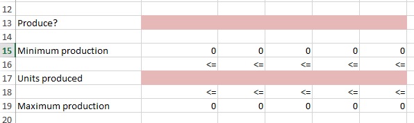
Below is a nice simple problem. We are building 2 types of furniture, tables and chairs. We are given the material and labor each item requires and the available amounts of each. We also have the profit per unit each item brings in. Our goal is to maximize profit. What we need to find out is how many of each item to build.

As you can see, this problem has already been solved using Excel Solver. Let’s see how we would approach this using PHPSimplex.

phpsimplex1.jpg

Go to the webite and click on the icon in the left corner or PHPSimplex in the menu bar.

phpsimplex2.jpg

I am going to select the Simplex/ Two Phases Method for this example

phpsimplex3.jpg

And based on our problem, I am going to choose 2 decision variables (my 2 pink changing cells) and two constraints (I will explain)

Now I am going to Maximize my function (I want max profits). Then I will set my function to 6X1+8X2 – The X1 and X2 represent my 2 changing cells. The 6 and 8 I get from my profit per unit found in my spread sheet.

So to put it in English : Max Profit = $6 * # of Tables Built + $8 * # of Chairs Built

phpsimplex5.jpg

Now our Constraints:

30X1 + 20X2 <= 300 – Materials – 30 * # Tables + 20 * # Chairs can’t exceed 300

5X1 + 10X2 <= 110 – Labor – 5 * # Tables + 10 * # Chairs can’t exceed 110

phpsimplex6.jpg

Now you can hit Continue  and PHPSimplex will step you through the process or you can just hi Direct Solution to get an answer. Let’s do that.

phpsimplex7.jpg

If you compare t he results below with the results I got from above using Excel Solver you will see they are the same.

phpsimplex8.jpg

Bottom Line

This is just a quick glimpse at what PHPSimplex offers. It is a fun site with lots of great information. If you want to dig deep and really learn how the process works mathematically, this is the site for you.

I highly recommend visiting their site.

Here is the link again: http://www.PHPSimplex.com/en/index.htm

Linear Optimization Model: Binary Constraints

Today we are going to build a Linear Optimization Model with binary constraints. What that means is that some of our decision variables are going to be restricted to 0 or 1 as possibilities.

This example is more complicated than earlier lessons, so I have included a fully filled out Excel file for you to follow along with. You can download the Excel file here: ModelBuild

Let’s start with the problem:

You have been hired by a company that builds airplane model kits. They currently produce 5 types of models – F-16’s, F-18’s, A-10’s, B-2’s, and B-52’s. They want you to help them maximize their profits.

They have provided you with the following production information.

The Minimum production may need a little explanation. Setting up the equipment to build a particular model has an expense built in. To cover that expense, you need to commit to building at least the value found in the minimum production row. If you can’t meet this level of production, we are not going to build any of this model.

binary1.jpg

We have also been given our available resources:

binary2.jpg

So now on to our decision variables. For each model, we have to first decide whether or not to produce. Remember, if we can’t produce our minimum amount for a particular model, we can’t produce any of that model.

So our Produce? decision variables are going to be either 1 (produce) or 0 (don’t produce)

binary3.jpg

Now our Minimum production row is a simple formula= Minimum production from row 7 above * your 1 or 0 from Produce?  I have placed a 1 in the first column of our Produce? row to demonstrate below.

binary4

Skip Units produced for now. Look at Maximum produced. This formula is simply the 1 or 0 from our Produce? row * 9999. I choose 9999 at random as I know we will never exceed this limit in our example. In other models, you may need a larger number.

Now Units produced is our second decision variable. This variable needs to sit in between Minimum production and Maximum production.

Note that if our Produce? variable is 0 (don’t build) Maximum production will be 0 (Produce? * 9999= 0) . Since Units produced needs to be less than or equal to Maximum production, we cannot produce any units.

Second, since if we decide to build (1), our Minimum production will come from our given values in blue. So our Units produced will need to be greater than or equal to the Minimum production.


Now lets set our Resource used using SUMPRODUCT()

Press Time

binary9.jpg

Grams Plastic

binary10

Finally, we need to set our Result cell – We do this using Sumproduct()

binary5.jpg

Now we can set up our solver.

  • Objective – Profit cell
  • Changing cells – our pink rows – note you separate the two rows with a comma
  • Set our Produce? row to binary (see second picture below)
  • Set Units produced to >= Minimum production
  • Set Units produced to <= Maximum production
  • Set Press Time Resource used <= Resource available
  • Set Grams Plastic Resource used <= Resource available

binary6

binary7.jpg


Finally make sure you are set to Simplex LP and hit Solve

binary8.jpg


R: Simple Linear Regression

Linear Regression is a very popular prediction method and most likely the first predictive algorithm most be people learn. To put it simply, in linear regression you try to place a line of best fit through a data set and then use that line to predict new data points.

linear1

If you are new to linear regression or are in need of a refresher, check out my lesson on Linear Regression in Excel where I go much deeper into the mechanics: Linear Regression using Excel

Get the Data

You can download our data set for this lesson here: linear1

Let’s upload our file into R

df <- read.csv(file.choose())
head(df)

linReg1

Now our data file contains a listing of Years a person has worked for company A and their Salary.

Check for linear relationship

With a 2 variable data set, often it is quickest just to graph the data to check for a possible linear relationship.

#plot data
attach(df)
plot(Years, Salary)

Looking at the plot, there definitely appears to be a linear relationship. I can easily see where I could draw a line through the data.

linReg2.jpg

An even better way to do it is to check for correlation. Remember the closer to 1, the better the correlation found in the data.

#check for correlation
cor(Years, Salary)

linReg3.jpg

Since our correlation is so high, I think it is a good idea to perform an linear regression.

Linear Regression in R

A linear regression in R is pretty simple. The syntax is lm(y, x, data)

#perform linear regression
fit <- lm(Salary~Years, data= df)
summary(fit)

linReg4.jpg

Now let’s take a second to break down the output.

The red box shows my P values. I want to make sure they are under my threshold (usually 0.05). This becomes more important in multiple regression.

The orange box shows my R-squared values. Since this is a simple regression, both of these numbers are pretty much the same, and it really doesn’t matter which one you look at. What these numbers tell me is how accurate my prediction line is. A good way to look at them for a beginner is to consider them to be like percentages. So in our example, our prediction model is 75-76% percent accurate.

Finally, the blue box are your coefficients. You can use these numbers to create your predictive model. Remember the linear equation: Y = mX + b? Well using your coefficients here our equation now reads Y = 1720.7X + 43309.7

Predictions

You can use fitted() to show you how your model would predict your existing data

fitted(fit)

linReg5.jpg

You can also use the predict command to try a new value

predict(fit, newdata =data.frame(Years= 40))

linReg7

Let’s graph our regression now.

plot(Years, Salary)

abline(fit, col = 'red')

linReg8

The Residuals Plot

I am not going to go too deep into the weeds here, but I want to show you something cool.

layout(matrix(c(1,2,3,4),2,2))  # c(1,2,3,4) gives us 4 graphs on the page, 

                                #2,2 - graphs are 2x2
plot(fit)

I promise to go more into this in a later lesson, but for now, I just want you to note the numbers you see popping up inside the graphs. (38,18,9) – These represent outliers. One of the biggest problems with any linear system is they are easily thrown off by outliers. So you need to know where you outliers are.

linReg9.jpg

If you look at the points listed in your graphs in your data, you will see why these are outliers. Now while this doesn’t tell you what to do about your outliers, that decision has to come from you, it is a great way of finding them quickly.

linReg10.jpg

The Code

# upload file
df <- read.csv(file.choose())
head(df)

#plot data
attach(df)
plot(Years, Salary)

#check for correlation
cor(Years, Salary)

#perform linear regression
fit <- lm(Salary~Years, data= df)
summary(fit)

#see predictions
fitted(fit)

predict(fit, newdata =data.frame(Years= 40))

#plot regression line 
plot(Years, Salary)

abline(fit, col = 'red')

layout(matrix(c(1,2,3,4),2,2)) 
plot(fit)

df


Python: Naive Bayes’

Naive Bayes’ is a supervised machine learning classification algorithm based off of Bayes’ Theorem. If you don’t remember Bayes’ Theorem, here it is:

bayes

Seriously though, if you need a refresher, I have a lesson on it here: Bayes’ Theorem

The naive part comes from the idea that the probability of each column is computed alone. They are “naive” to what the other columns contain.

You can download the data file here: logi2

Import the Data

import pandas as pd
df = pd.read_excel("C:\Users\Benjamin\Documents\logi2.xlsx")
df.head()

nb.jpg

Let’s look at the data. We have 3 columns – Score, ExtraCir, Accepted. These represent:

  • Score – Student Test Score
  • ExtraCir – Was Student in an Extra Circular Activity
  • Accepted – Was the Student Accepted

Now the Accepted column is our result column – or the column we are trying to predict. Having a result in your data set makes this a supervised machine learning algorithm.

Split the Data

Next split the data into input(score and extracir) and results (accepted).

y = df.pop('Accepted')
X = df

y.head()

X.head()

nb1.jpg

Fit Naive Bayes

Lucky for us, scikitlearn has a bit in Naive Bayes algorithm – (MultinomialNB)

Import MultinomialNB and fit our split columns to it (X,y)

from sklearn.naive_bayes import MultinomialNB
classifier = MultinomialNB()
classifier.fit(X,y)

nb2.jpg

Run the some predictions

Let’s run the predictions below. The results show 1 (Accepted) 0 (Not Accepted)

#--score of 1200, ExtraCir = 1
print(classifier.predict([1200,1]))

#--score of 1000, ExtraCir = 0
print(classifier.predict([1000,0]))

nb3

The Code

import pandas as pd
df = pd.read_excel("C:\Users\Benjamin\Documents\logi2.xlsx")
df.head()

y = df.pop('Accepted')
X = df

y.head()
X.head()

from sklearn.naive_bayes import MultinomialNB
classifier = MultinomialNB()
classifier.fit(X,y)

#--score of 1200, ExtraCir = 1
print(classifier.predict([1200,1]))

#--score of 1000, ExtraCir = 0
print(classifier.predict([1000,0]))


Bayes’ Theorem

Bayes’ Theorem sits at the heart of a few well known machine learning algorithms. So a fundamental understanding of the theorem is in order.

Let’s consider the following idea (the following stats are completely made up by the way). Imagine 5% of kids are dyslexic. Now imagine the tests administered for dyslexia at a local school is known to give a false positive 10% of the time. What is the probability a kid has dyslexia given the fact they tested positive?

What we want to know is = P(Dyslexic | Positive Test).

To figure this out, we are going to use Bayes’ Theorem

Let’s start with the equation:

bayes

Don’t worry. It is not all that complicated. Let’s break it down into parts:

  • P(A) and P(B) are the probabilities of A or B happening independent of each other
  • P(A|B) is the probability of A given the B has occurred
  • P(B|A) is the probability of B given that A has occurred

Let’s take a new look at the formula

bayes6.jpg

So let me put this into English.

  • P(Dyslexic|Positive Test) = probability the kid is dyslexic assuming he has positive test
  • P(Dyslexic) = the probability the kid being dyslexic
  • P(Positive Test) = Probability of a positive test
  • P(Positive Test |Dyslexic) = The probability positive test assuming the kid is dyslexic


First, let’s figure out our probabilities. A tree chart is a great way to start.

Look at the chart below. It branches first between dyslexic and not dyslexic. Then each branch has positive and negative probabilities branching from there.

bayes4

Now to calculate the probabilities. We do this by multiplying the branches. For example Dyslexic and Positive  0.05 * 0.9 = 0.045

bayes5.jpg

Now, let’s fill in our formula. If you are having trouble seeing where the values come from look at the chart below

  • P(Pos test | Dyslexic) = red * green = 0.05*0.9=.0.045
  • P(Dyslexic) = First section of top branch = 0.05
  • P(Positive Test) = red*green + yellow * yellow = 0.05*0.9+0.95*0.1=0.045+0.095

bayes8.jpg

bayes7.jpg

So the probability of being dyslexic assuming the kid had a positive test = 0.016 or 1.6%


Another – perhaps more real world use for Bayes’ Theorem is the SPAM filter. Check it out below. See if you can figure your way through it on your own.

bayes3


  • P(SPAM|Words) – probability an email is SPAM based on words found in the email
  • P(SPAM) – probability of an email being SPAM in general
  • P(Words) – probability of words appearing in email
  • P(Words|SPAM) – probability of words being in an email if we know it is SPAM

Probability: An Introduction

Many popular machine learning algorithms are based on probability. If you are a bit shaky on your probability, don’t worry this quick primer will get you up to speed.

Think about a coin flip. There are 2 possibilities you could have (heads or tails). So if you wanted to know the probability of getting heads in any particular flip, it would be 1/2 (desired outcome/all possible outcomes).

Now take a 6 sided die:

  • The probability rolling a 1 is 1/6.
  • rolling an even number (2,4,6) = 3/6 or 1/2
  • rolling a number less than 3 (1,2) = 2/6 or 1/3

The compliment of a probability can also be referred to the probability of an event NOT happening. The probability of not rolling a 1 on a six sided die = 5/6.

P(~A) = 1 – P(A) = 1 – 1/6 = 5/6

Independent Probability

Independent probability simply means determining the probability of 2 or more events when the outcome of one event has no effect on the other.

Let’s take two coins (A and B). Take the first coin and flip it. Imagine it comes up heads. Now flip the second coin. The fact that the first coin can up heads will not influence the outcome of the second flip in any way. To show this mathematically:

  • Probability of flipping heads coin A = P(A) = 1/2
  • Probability of flipping heads coin B = P(B) = 1/2
  • Probability of flipping 2 heads = P(A and B) = P(A ∩ B) = P(A)*P(B)=1/2*1/2=1/4

Mutually Exclusive

Now we are asking if event A or B occurred.

P(A or B) = P(A∪B) = P(A) +P(B)

So the probability of 10 or a 2 from a deck of cards = 1/52 + 1/52 = 2/52 = 1/26

Not Mutually Exclusive

Imaging drawing an Ace and a Red Card. We want to make sure to factor in all the elements, but we need to account for double counting.

P(A or B) = P(A∪B) = P(A) +P(B) – P(A and B)

4/52 (ACE) + 26/52(Red Card) – 2/52(To get both an Ace and a Red card, the only options are Ace of Hearts and Ace of Diamonds) = 28/52 = 7/13

Conditional Probability

Now we are going to work with dice. One six sided die and one 4 sided die. The diagram below shows all 24 possible combinations.

prob.jpg

Now conditional probability is the probability of something occurring assuming some prior event has occurred.  Look at the chart above, lets consider the A = rolling even number on six sided die (3/6) and B = rolling even number on 4 side die(2/4). So P(A|B) (read probability of A given B) = P(A∩B)/P(B). Lets look a the chart to help use see this.

prob1

So, when rolling a six sided die (A), you have a 3/6 chance of rolling an even number(2,4,6)

When rolling a four sided die (B), you have a 2/4 chance of rolling an even number(2,4)

So P(A and B)  = 3/6*2/4=6/24=1/4

Now when figuring P(A|B) (rolling an even on the four side die assuming you have already rolled an even on the six sided die) we are no longer looking at all 24 combinations, we are now only looking at the combination where the six side die (A) is even (the green columns). So as you can see, of the 12 options where A is even, 6 have an even number on the 4 sided die.

So… P(A ∩ B)/P(B) = (1/4)/(1/2) = 1/2. Which makes sense since of the 12 combinations where A is even, 6 have even numbers for B. 6/12 = 1/2

Python: K Means Clustering Part 2

In part 2 we are going focus on checking our assumptions. So far we have learned how to perform a K Means Cluster. When running a K Means Cluster, you first have to choose how many clusters you want. But what is the optimal number of clusters? This is  the “art” part of an algorithm like this.

One thing you can do is check the distance from you points to the cluster center. We can measure this using the interia_ function from scikit learn.

Let’s start by building our K Means Cluster:

Import the data

import pandas as pd

df = pd.read_excel("C:\Users\Benjamin\Documents\KMeans1.xlsx")
df.head()

kmeans1

Drop unneeded columns

df1 = df.drop(["ID Tag", "Model", "Department"], axis = 1)
df1.head()

kmeans2

Create the model – here I set clusters to 4

from sklearn.cluster import KMeans
km = KMeans(n_clusters=4, init='k-means++', n_init=10)

Now fit the model and run the interia_ function

km.fit(df1)
km.inertia_

kmeaninter.jpg

Now the answer you get is the sum of distances from your sample points to the cluster center.

What does the number mean? Well, on its own, not much. What you need to do is look at a list of interia_ for a range of cluster choices.

To do so, I am set up a for loop.

n = int(raw_input("Enter Starting Cluster: "))
n1 = int(raw_input("Enter Ending Cluster: "))
for i in range(n,n1):
 km = KMeans(n_clusters=i, init='k-means++', n_init=10)
 km.fit(df1)
 print i, km.inertia_

kmeaninter1.jpg

The trick to reading the results is look for the point of diminishing returns. The area I am pointing to with the arrow is where I would look. The changes in values start slowing down here.

I am using this example because I feel it is more real world. Working with real data takes time to a get a feeling for. If you are having trouble seeing why I chose this point, consider the following textbook example:

See how at this highlight part, the drop in number goes from hundreds to 25. That is a diminished return. The new result is not that much better than the earlier result. As opposed to 1 and 2 where 2 clusters perform 1000 units better.

kmeaninter2.jpg


R: ggplot using facets

In this example I am going to teach you to use facets to add another level to your ggplot data visualizations. In this example we will be working with the ChickWeight data set from R Datasets

First, let’s check out the data by running head()

head(ChickWeight)

facet1.jpg

We have 4 columns in our data, weight, Time, Chick, and Diet.

Now, let’s build our ggplot model. Below, we are setting our model to a variable “p1”. We then set ChickWeight as our data set and the weight column to our x axis. Remember, nothing will happen when running the line below.

p1 <- ggplot(data=ChickWeight, aes(x=weight))

Now lets graph our plot as a histogram – we will set our binwidth to 10 – if any of this confusing you, go back and check out my earlier lessons on ggplot and ggplot histograms

p1 + geom_histogram(binwidth = 10)

facet2.jpg

Let’s now add some color. I am going to set our “fill” to be Diet

p1 + geom_histogram(binwidth = 10, aes(fill=Diet))

facet3.jpg

Now, using facets, I am going to take it one step further and separate this into 4 histograms, one for each diet.

 p1 + geom_histogram(binwidth = 10, aes(fill=Diet)) + facet_grid(Diet~.)

facet4.jpg

The Code

#-- Look at data

head(ChickWeight)

#-- build ggplot model
p1 <- ggplot(data=ChickWeight, aes(x=weight))

#--plot ggplot as histogram
p1 + geom_histogram(binwidth = 10)

#-- set fill color to Diet
p1 + geom_histogram(binwidth = 10, aes(fill=Diet))

#-- create four histograms - one for each Diet
p1 + geom_histogram(binwidth = 10, aes(fill=Diet)) + facet_grid(Diet~.)


Probability vs Odds

Probability and odds are constantly being misused. Even in respected publications you will see sentences such as: “The odds of a Red Sox win tonight is 60%.” or “His probability is 2 to 1.” While in the lexicon of American English these words seem to have taken on interchanging meaning, when working with statisticians or data scientists, you are going to want to get your vocabulary straight.

Probability:

Probability is a number between 0 and 1, often represented as a fraction or percentage. The probability is determined by dividing the number of positive outcomes by the total number of possible outcomes. So if you have 4 doors and 1 has a prize behind it, your probability of picking the right door is 1/4 or 0.25 or 25%.

Note, do not let the term positive outcome confuse you. It is not a qualifier of good vs bad or happy vs sad. It simply means the result is what you are looking for based on the framing of your question. If I were to state that out of every 6 patients who opt for this new surgery 2 die – 2 would be the “positive outcome” in my equation (2/6 or approx 33%) even though dying is far from a “positive outcome”.

Odds:

Odds, on the other hand, are a ratio. The odds of rolling a 4 on a six sided die is 1:5 (read 1 in 5). The odds ratio works like this: positive outcomes : negative outcomes. So the odds of rolling an even number on a six sided die is 3:3 (or simplified to 1:1).

Now the probability of rolling an even number on a six sided die is 3/6 or 1/2. So keep that in mind, odds of 1:2 is actually a probability of 1/3 not 1/2.

Deck of Cards:

Working with a standard deck of playing cards (52 cards).

Pulling a Red card from the deck

  • probability: 26/52 = 1/2
  • odds: 26:26 = 1:1

Pulling an Ace from the deck

  • probability: 4/52 = 1/13
  • odds: 4:48 = 1:12

Pulling a Diamond from the deck

  • probability: 13/52 = 1/4
  • odds: 13:39 = 1:3