
Before you can do anything with your data, it has to be cleaned and prepped. While certain fixes (spelling errors, date format, number format, etc.) are easy enough to handle, merging multiple tables or worksheets together can be frustrating. I have witnessed seasoned Excel users reduced to manually inputting hundreds of data fields into their spreadsheet. If only they knew how to use the look up functions built into Excel.
Vlookup
Vlookup (and its transposed partner Hlookup) are 2 of the most common look up functions in Excel. And while they may seem complex at first, they are actually pretty easy to use.
Enough talk though, let us see how it works:

Here are two tables from an imaginary auto repair shop. The Green Table shows a list of work orders, while the Yellow Table shows a pricing list for the services the shop offers. So, the task at hand is to use the Yellow Table to populate a price column on the Green Table.
Start simply enough, go to the last column of the Green Table Right Click > Insert Column. Name the column Price and go to the first open cell in the column and input the following formula: =VLOOKUP(D2,$G$2:$H$&,2,FALSE)

Now I know this looks complicated, but I promise it is not as bad as it looks.
- Start with =VLOOKUP() **Whenever = is the first character in a cell, Excel automatically knows what follows is a formula.
- The first element inside the parenthesis of a VLOOKUP is the reference cell in your main table. In the example above, I chose cell D2 (seen in blue), which holds the service information for the first work order. This is the data field I want to reference against my lookup table.
- The next element is the range of the lookup table (seen in red). The lookup table range in this example is G2:H7. **After highlighting the lookup table, select F4 to lock the range in $G$2:$H$7. This ensures that as the VLOOKUP formula is replicated down the sheet, the lookup table stays locked in place.
- The next element in the formula is the column that holds the return value. We are looking for the price from the Yellow Table, so column 2 holds the return value.
- The final element is Exact or Closest Match. FALSE means only exact matches. TRUE means closest matches.
Once the formula is complete, hit enter and the price will appear in the cell. Finally, replicate the formula down through all Work Order records in the Green Table.

Excel tip: If you hover your mouse over the little green square the arrow is pointing to, your cursor will become a black plus sign. Double click on the green square and the formula will be replicated down all the remaining rows in your table.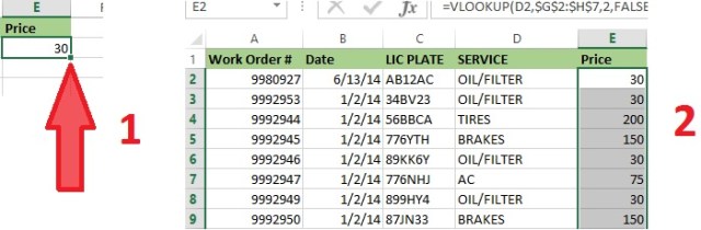

Pingback: Merging Data with Excel | SutoCom Solutions
I’ll right away seize your rss as I can’t in finding your
e-mail subscription link or e-newsletter service. Do you’ve any?
Kindly permit me recognize so that I may just subscribe.
Thanks.
Amy, thank you for your comment. Sorry about not having an email subscription up. This blog is new, and I must have overlooked it. I have added an email subscription link to the site now. It is in the left column of the page.